COVID-19 en población pediátrica menor de 18 años según registros nacionales en Perú, 2020-2023

Brian Norman Peña-Calero

In [1]:

library(tidyverse)

Warning: package 'purrr' was built under R version 4.4.3

── Attaching core tidyverse packages ──────────────────────── tidyverse 2.0.0 ──
✔ dplyr     1.1.4     ✔ readr     2.1.5
✔ forcats   1.0.0     ✔ stringr   1.5.1
✔ ggplot2   3.5.1     ✔ tibble    3.2.1
✔ lubridate 1.9.4     ✔ tidyr     1.3.1
✔ purrr     1.0.4     
── Conflicts ────────────────────────────────────────── tidyverse_conflicts() ──
✖ dplyr::filter() masks stats::filter()
✖ dplyr::lag()    masks stats::lag()
ℹ Use the conflicted package (<http://conflicted.r-lib.org/>) to force all conflicts to become errors

library(arrow)

Warning: package 'arrow' was built under R version 4.4.3


Adjuntando el paquete: 'arrow'

The following object is masked from 'package:lubridate':

    duration

The following object is masked from 'package:utils':

    timestamp

library(duckdb)

Warning: package 'duckdb' was built under R version 4.4.3

Cargando paquete requerido: DBI

library(dbplyr)


Adjuntando el paquete: 'dbplyr'

The following objects are masked from 'package:dplyr':

    ident, sql

library(innovar)
library(apyramid)
library(sf)

Linking to GEOS 3.12.2, GDAL 3.9.3, PROJ 9.4.1; sf_use_s2() is TRUE

library(lmerTest)

Cargando paquete requerido: lme4
Cargando paquete requerido: Matrix

Adjuntando el paquete: 'Matrix'

The following objects are masked from 'package:tidyr':

    expand, pack, unpack


Adjuntando el paquete: 'lmerTest'

The following object is masked from 'package:lme4':

    lmer

The following object is masked from 'package:stats':

    step

library(emmeans)

Warning: package 'emmeans' was built under R version 4.4.3

Welcome to emmeans.
Caution: You lose important information if you filter this package's results.
See '? untidy'

source("03_functions/index_calculator.R")
source("03_functions/compare_levels_per_month.R")

Disponibilidad de los datos

In [2]:

con <- dbConnect(duckdb(), dbdir = "01_data/raw/covid.duckdb", read_only = TRUE)

vacunas <- tbl(con, "vacunas")
vacunas_18 <- tbl(con, "vacunas_18")
fallecidos_total <- tbl(con, "fallecidos_total")
positivos <- tbl(con, "positivos")
positivos_0723 <- tbl(con, "positivos_0723")
hospitalizados <- tbl(con, "hospitalizados")
hosp_final <- tbl(con, "hosp_final")
poblacion <- tbl(con, "poblacion")
peru_mother <- tbl(con, "peru_mother")
# pobreza <- tbl(con, "pobreza")
data(Peru)

In [3]:

fallecidos_summary <- fallecidos_total %>% 
  summarise(
    n = n(),
    min = min(fecha_fallecimiento),
    max = max(fecha_fallecimiento)
  ) %>% 
  collect()

Warning: Missing values are always removed in SQL aggregation functions.
Use `na.rm = TRUE` to silence this warning
This warning is displayed once every 8 hours.

positivos_summary <- positivos %>% 
  summarise(
    n = n(),
    min = min(fecha_resultado),
    max = max(fecha_resultado)
  ) %>% 
  collect() 

hospitalizados_summary <- hospitalizados %>% 
  summarise(
    n = n(),
    min = min(fecha_ingreso_hosp),
    max = max(fecha_ingreso_hosp)
  ) %>% 
  collect() 

vacunas_summary <- vacunas %>% 
  summarise(
    n = n(),
    min = min(fecha_vacunacion),
    max = max(fecha_vacunacion)
  ) %>% 
  collect() %>% 
  mutate(
    across(min:max,
           ymd)
  )

max_positivos_0723 <- positivos_0723 %>% 
  summarise(max = max(fecha_resultado)) %>% 
  pull(max)

Peru <- Peru %>%  
  left_join(
    peru_mother %>% 
      as_tibble()
  )

Joining with `by = join_by(ubigeo, dep, prov, distr)`

peru_dep_sf <- Peru %>%
  group_by(dep.code, dep) %>%
  summarise() %>% 
  ungroup()

`summarise()` has grouped output by 'dep.code'. You can override using the
`.groups` argument.

peru_reg_sf <- Peru %>%
  group_by(region) %>%
  summarise() %>% 
  ungroup()

peru_macro_sf <- Peru %>%
  group_by(macrorregion) %>%
  summarise() %>% 
  ungroup()

Actualmente los datos disponibles para el análisis tienen las siguientes situaciones:

Fallecidos COVID-19: Ahora mismo, esta data (Fallecidos por COVID-19 - [Ministerio de Salud - MINSA]) se encuentra actualizada en el portal de datos abiertos. Cuenta con 220 816 fallecidos que van desde 2020-03-03 al 2024-02-03.
Casos positivos COVID-19: Esta base de datos ya fue corregida y actualizada recientemente en la plataforma de datos abiertos. Cuenta con 4 548 255 casos positivos que van desde 2020-03-06 al 2023-12-31. Sin embargo, tiene el inconveniente de no tener registrado el id_persona que es indispensable para poder calcular los casos nuevos positivos COVID-19. Se usará por ahora una base actualizada a junio del 2023 con algunos casos menos, pero que si tiene esta información. El enlace de descarga de esa data desde el mismo Minsa ya no se encuentra disponible, pero si está en este repositorio Github: https://github.com/jmcastagnetto/covid-19-peru-limpiar-datos-minsa/tree/main/datos/originales
Hospitalizados por COVID-19: Esta data contiene a la vez información de la vacunación y fallecimiento de quienes fueron hospitalizados. Cuenta con 150 791 casos hospitalizados que van desde 2019-06-06 al 2024-01-03.
Vacunación COVID-19: Esta data contiene información de vacuna. Cuenta con 91 838 312 registros de vacunación que van desde 2020-04-27 al 2023-12-30.
Población Estimada: Esta data contiene las estimaciones poblacionales desde el 2020 al 2023 realizada por REUNIS. Presenta subdivisiones por distrito, edad y sexo. Sin embargo, la versión del año 2021, no tiene subdivisión por sexo, por lo que se usa la estimación realizada por el INEI que si lo contiene.

Para términos de uniformidad, temporalmente se restringirán todos los datos a junio de 2023.

Positivos - Prevalencia COVID-19

Para la estimación de la prevalencia, se obtuvo los datos poblacionales por distrito, sexo y grupo de edad para 2020, 2021, 2022 y 2023. A partir de ello, se calculó una prevalencia promedio mensual (Ecuación 1) que luego fue promediada para obtener un único valor por distrito, sexo y grupo de edad. Finalmente, se reporta la prevalencia promedio mensual por 1000 habitantes en anualidades (Ecuación 2) u olas covid, a fin de tener una lectura con menor términos decimales.

\[ \text{Prevalencia promedio mensual}_i = \frac{\text{Promedio de Número de casos en el mes del año } i}{\text{Población en el año } i} \tag{1}\]

Donde:

\(\text{Número de casos en el año } i\) es el número de positivos COVID-19 en un año en específico (2020-2023)
\(\text{Población en el año } i\) es la población que puede ser afectada por COVID-19 en un año en específico (2020-2023)

\[ \text{Prevalencia Promedio mensual por 1000 habitantes} = \left( \frac{\sum_{i=2020}^{2023} \text{Prevalencia promedio mensual}_i}{\text{Número de Años}} \right) \times 1000 \tag{2}\]

Vista general

In [4]:

positivos_0723 <- positivos_0723 %>% 
  filter(edad < 18, 
         sexo != "No registrado") %>% 
  mutate(
    overall = "overall"
  ) 

range_pos_18_0723 <- positivos_0723 %>% 
  summarise(
    min = min(fecha_resultado),
    max = max(fecha_resultado)
  ) %>% 
  collect() %>% 
  mutate(
    min = format(min, "%d-%m-%Y"),
    max = format(max, "%d-%m-%Y"),
    fecha = paste0("(", min, " a ", max, ")")
  )

In [5]:

levels <- list(
  c("overall"),
  c("grupo_edad"),
  c("sexo"),
  c("ola_covid"),
  c("ola_covid", "grupo_edad"),
  c("ola_covid", "sexo"),
  c("ola_covid", "region"),
  c("ola_covid", "macrorregion"),
  c("departamento"),
  c("departamento", "sexo"),
  c("departamento", "grupo_edad"),
  c("departamento", "sexo", "grupo_edad"),
  c("departamento", "ola_covid"),
  c("distrito"),
  c("distrito", "sexo"),
  c("distrito", "grupo_edad"),
  c("distrito", "cuartil_pobreza"),
  c("grupo_edad", "cuartil_pobreza"),
  c("sexo", "cuartil_pobreza"),
  c("ola_covid", "cuartil_pobreza"),
  c("ola_covid", "cuartil_nbi"),
  c("cuartil_pobreza"),
  c("cuartil_nbi"),
  c("region"),
  c("macrorregion")
)

# Calcular la prevalencia
results_prevalencia <- index_calculator(
  data = positivos_0723,
  denom = poblacion %>% mutate(overall = "overall"), 
  levels = levels, 
  type = "month"
)

results_per_month_prevalencia <- index_calculator(
  data = positivos_0723,
  denom = poblacion %>% mutate(overall = "overall"),
  levels = levels, 
  type = "per_month"
)

In [6]:

positivos_0723_tbl <- positivos_0723 %>% 
  select(edad, overall, grupo_edad, sexo, ola_covid, region, 
         macrorregion, cuartil_pobreza, cuartil_nbi) %>% 
  collect()

labelled::var_label(positivos_0723_tbl) <- list(
  overall = "Overall",
  grupo_edad = "Age Group",
  sexo = "Sex",
  ola_covid = "COVID-19 wave",
  region = "Natural Regions",
  macrorregion = "Macroregions",
  cuartil_pobreza = "Poverty level",
  cuartil_nbi = "Unsatisfied basic needs level"
)

In [7]:

tbl_summ_positivos <- positivos_0723_tbl %>% 
  select(-edad) %>% 
  gtsummary::tbl_summary(
    type = list(
      overall ~ "dichotomous"
    ),
    value = list(overall = "overall"),
    missing_text = "No data"
  ) %>% 
  gtsummary::modify_header(label = "**Variables**") %>%
  gtsummary::bold_labels()

tbl_summ_positivos_c2 <- results_prevalencia$overall$index %>% 
  mutate(label = "Overall") %>% 
  rename(variable = overall) %>% 
  bind_rows(
    results_prevalencia$grupo_edad$index %>% 
      mutate(variable = "grupo_edad") %>% 
      rename(label = grupo_edad),
    results_prevalencia$sexo$index %>% 
      mutate(variable = "sexo") %>% 
      rename(label = sexo),
    results_prevalencia$ola_covid$index %>% 
      mutate(variable = "ola_covid") %>% 
      rename(label = ola_covid),
    results_prevalencia$region$index %>% 
      mutate(variable = "region") %>% 
      rename(label = region),
    results_prevalencia$macrorregion$index %>% 
      mutate(variable = "macrorregion") %>% 
      rename(label = macrorregion),
    results_prevalencia$cuartil_pobreza$index %>% 
      mutate(variable = "cuartil_pobreza") %>% 
      rename(label = cuartil_pobreza),
    results_prevalencia$cuartil_nbi$index %>% 
      mutate(variable = "cuartil_nbi") %>% 
      rename(label = cuartil_nbi)
  ) %>% 
  drop_na() %>% 
  mutate(
    rate = formattable::digits(rate, 3)
  )


tbl_summ_positivos_final <- tbl_summ_positivos %>%
  gtsummary::modify_table_body(
    ~ .x %>% 
      left_join(tbl_summ_positivos_c2) %>% 
      mutate(
        label = case_when(
          variable %in% c("cuartil_pobreza", "cuartil_nbi") &
            label == "1" ~ "1 (0-19.9%)",
          variable %in% c("cuartil_pobreza", "cuartil_nbi") & 
            label == "2" ~ "2 (20-39.9%)",
          variable %in% c("cuartil_pobreza", "cuartil_nbi") & 
            label == "3" ~ "3 (40-59.9%)",
          variable %in% c("cuartil_pobreza", "cuartil_nbi") &
            label == "4" ~ "4 (60-100%)",
          .default = label
        )
      )
  ) %>% 
  gtsummary::modify_header(
    rate ~ "**Average monthly prevalence per 1000 inhabitants**"
  )

Joining with `by = join_by(variable, label)`

In [8]:

tbl_summ_positivos_final

Tabla 1: Descriptivos de casos positivos menores de 18 años (07-03-2020 a 17-06-2023)

Variables	N = 315,046¹	Average monthly prevalence per 1000 inhabitants
Overall	315,046 (100%)	0.810
Age Group
Under 1 year	16,537 (5.2%)	0.826
1 - 5 years	45,573 (14%)	0.413
6 - 11 years	91,657 (29%)	0.706
12 - 17 years	161,279 (51%)	1.252
Sex
Female	159,581 (51%)	0.824
Male	155,465 (49%)	0.796
COVID-19 wave
1 (Mar – Oct 2020)	59,889 (19%)	0.782
2 (Nov 2020 – Oct 2021)	72,471 (23%)	0.592
3 (Nov 2021 – Apr 2022)	106,291 (34%)	1.844
4 (May 2022 – Oct 2022)	58,179 (18%)	1.016
5 (Nov 2022 – Jun 2023)	18,143 (5.8%)	0.235
No data	73
Natural Regions
Coast	234,478 (74%)	1.008
Highlands	53,944 (17%)	0.488
Jungle	26,624 (8.5%)	0.578
Macroregions
Center	72,047 (23%)	0.833
East	24,421 (7.8%)	0.555
Metropolitan Lima and Callao	118,357 (38%)	1.126
North	50,563 (16%)	0.564
South	49,658 (16%)	0.784
Poverty level
1 (0-19.9%)	233,362 (78%)	1.062
2 (20-39.9%)	49,734 (17%)	0.485
3 (40-59.9%)	15,063 (5.0%)	0.287
4 (60-100%)	1,476 (0.5%)	0.138
No data	15,411
Unsatisfied basic needs level
1 (0-19.9%)	189,560 (63%)	1.118
2 (20-39.9%)	80,980 (27%)	0.586
3 (40-59.9%)	17,980 (6.0%)	0.334
4 (60-100%)	11,115 (3.7%)	0.403
No data	15,411
¹ n (%)

In [9]:

tbl_summ_positivos_final %>% 
  gtsummary::as_hux_xlsx("02_output/tables/positivos_descriptivos.xlsx")

tbl_summ_positivos_final %>%
  gtsummary::as_flex_table() %>%
  flextable::save_as_docx(path = "02_output/tables/positivos_descriptivos.docx")

In [10]:

downloadthis::download_file(
  path = "02_output/tables/positivos_descriptivos.xlsx",
  button_label = "Descargar tabla en Excel",
  button_type = "success",
  has_icon = TRUE,
  icon = "fa fa-save"
)

In [11]:

downloadthis::download_file(
  path = "02_output/tables/positivos_descriptivos.docx",
  button_label = "Descargar tabla en Word",
  button_type = "primary",
  has_icon = TRUE,
  icon = "fa fa-save"
)

In [12]:

comparing_levels <- list(
  c("grupo_edad"),
  c("sexo"),
  c("ola_covid"),
  c("cuartil_pobreza"),
  c("cuartil_nbi"),
  c("region"),
  c("macrorregion")
)

prevalence_comparisons <- compare_levels_per_month(
  results_per_month = results_per_month_prevalencia,
  levels = comparing_levels
)

# Extraer las tablas `cld` como tibbles, renombrando y añadiendo una columna "level"
prevalence_comparisons_cld_pre <- lapply(names(prevalence_comparisons), function(level) {
  cld <- prevalence_comparisons[[level]]$cld
  
  if (!is.null(cld)) {
    cld <- cld |> 
      as_tibble() |> 
      rename(group = 1) |>  # Renombra la primera columna a 'group'
      mutate(level = level) |> # Añade una columna 'level' con el nombre de la lista
      relocate(level) 
  }
  
  cld
}) |> 
  bind_rows()

prevalence_comparisons_cld_pre <- 
  prevalence_comparisons_cld_pre |> 
  mutate(
    across(
      where(is.numeric),
      ~ formattable::digits(.x, 3)
    )
  )

In [13]:

In [14]:

prevalence_comparisons_cld <- prevalence_comparisons_cld_pre |> 
  rename_with(
    .fn = ~ paste0("**", str_to_title(.x), "**")
  ) %>% 
  gt::gt() %>% 
  gt::cols_label(
    .fn = gt::md,
    .process_units = TRUE
  )

prevalence_comparisons_cld

Tabla 2: Comparaciones múltiples de incidencia(07-03-2020 a 17-06-2023)

Level	Group	Emmean	Se	Df	Lower.cl	Upper.cl	.Group
grupo_edad	1 - 5 years	0.413	0.206	52.745	-0.000	0.826	a
grupo_edad	6 - 11 years	0.706	0.206	52.745	0.293	1.119	ab
grupo_edad	Under 1 year	0.826	0.206	52.745	0.413	1.238	b
grupo_edad	12 - 17 years	1.252	0.206	52.745	0.839	1.664	c
sexo	Male	0.796	0.201	39.051	0.390	1.202	a
sexo	Female	0.824	0.201	39.051	0.418	1.230	b
ola_covid	5 (Nov 2022 – Jun 2023)	0.235	0.435	35.000	-0.648	1.118	a
ola_covid	2 (Nov 2020 – Oct 2021)	0.592	0.355	35.000	-0.129	1.313	a
ola_covid	1 (Mar – Oct 2020)	0.782	0.435	35.000	-0.101	1.665	a
ola_covid	4 (May 2022 – Oct 2022)	1.016	0.502	35.000	-0.004	2.035	a
ola_covid	3 (Nov 2021 – Apr 2022)	1.844	0.502	35.000	0.824	2.864	a
cuartil_pobreza	4	0.104	0.153	103.028	-0.199	0.407	a
cuartil_pobreza	3	0.287	0.149	97.243	-0.008	0.582	a
cuartil_pobreza	2	0.474	0.150	99.073	0.177	0.772	a
cuartil_pobreza	1	1.062	0.149	97.243	0.767	1.357	b
cuartil_nbi	3	0.334	0.170	83.048	-0.004	0.672	a
cuartil_nbi	4	0.389	0.171	84.741	0.049	0.729	a
cuartil_nbi	2	0.586	0.170	83.048	0.248	0.924	a
cuartil_nbi	1	1.118	0.170	83.048	0.780	1.456	b
region	Highlands	0.488	0.181	67.051	0.127	0.848	a
region	Jungle	0.578	0.181	67.051	0.218	0.939	a
region	Coast	1.008	0.181	67.051	0.648	1.369	b
macrorregion	East	0.555	0.204	54.864	0.145	0.965	a
macrorregion	North	0.564	0.204	54.864	0.154	0.974	a
macrorregion	South	0.784	0.204	54.864	0.374	1.194	ab
macrorregion	Center	0.833	0.204	54.864	0.423	1.243	ab
macrorregion	Metropolitan Lima and Callao	1.126	0.204	54.864	0.716	1.536	b

In [15]:

prevalence_comparisons_cld_pre %>% 
  rename_with(
    .fn = str_to_title
  ) %>% 
  huxtable::as_hux() %>% 
  huxtable::set_bold(1, 1:8) %>% 
  huxtable::quick_xlsx(file = "02_output/tables/prevalencia_comparacion_multiple.xlsx",
                       open = FALSE)

prevalence_comparisons_cld %>%
  gt::gtsave("02_output/tables/prevalencia_comparacion_multiple.docx")

In [16]:

downloadthis::download_file(
  path = "02_output/tables/prevalencia_comparacion_multiple.xlsx",
  button_label = "Descargar tabla en Excel",
  button_type = "success",
  has_icon = TRUE,
  icon = "fa fa-save"
)

In [17]:

downloadthis::download_file(
  path = "02_output/tables/prevalencia_comparacion_multiple.docx",
  button_label = "Descargar tabla en Word",
  button_type = "primary",
  has_icon = TRUE,
  icon = "fa fa-save"
)

In [18]:

tbl_summ_positivos_edad_ola <- positivos_0723_tbl %>% 
  select(-edad) %>% 
  gtsummary::tbl_summary(
    by = ola_covid,
    type = list(
      overall ~ "dichotomous"
    ),
    value = list(overall = "overall"),
    missing_text = "No data"
  ) %>% 
  gtsummary::modify_header(label = "**Variables**") %>%
  gtsummary::bold_labels()

73 missing rows in the "ola_covid" column have been removed.

ola_covid_positivos_gtsumm <- results_prevalencia$ola_covid$index %>% 
  rename(stat = ola_covid) %>% 
  mutate(label = "Overall",
         variable = "overall") %>% 
  bind_rows(
    results_prevalencia$ola_covid_grupo_edad$index %>%
      mutate(variable = "grupo_edad") %>% 
      rename(label = grupo_edad,
             stat = ola_covid),
    results_prevalencia$ola_covid_sexo$index %>% 
      mutate(variable = "sexo") %>% 
      rename(label = sexo,
             stat = ola_covid),
    results_prevalencia$ola_covid_region$index %>% 
      mutate(variable = "region") %>% 
      rename(label = region,
             stat = ola_covid),
    results_prevalencia$ola_covid_macrorregion$index %>% 
      mutate(variable = "macrorregion") %>%
      rename(label = macrorregion,
             stat = ola_covid),
    results_prevalencia$ola_covid_cuartil_pobreza$index %>% 
      mutate(variable = "cuartil_pobreza") %>% 
      rename(label = cuartil_pobreza,
             stat = ola_covid),
    results_prevalencia$ola_covid_cuartil_nbi$index %>% 
      mutate(variable = "cuartil_nbi") %>% 
      rename(label = cuartil_nbi,
             stat = ola_covid)
  ) %>% 
  mutate(
    rate = formattable::digits(rate, 3),
    stat = as.character(stat),
    stat = case_match(
      stat,
      "1 (Mar – Oct 2020)" ~ "stat_1",
      "2 (Nov 2020 – Oct 2021)" ~ "stat_2",
      "3 (Nov 2021 – Apr 2022)" ~ "stat_3",
      "4 (May 2022 – Oct 2022)" ~ "stat_4",
      "5 (Nov 2022 – Jun 2023)" ~ "stat_5"
    )
  ) 

tbl_summ_positivos_edad_ola$table_body <- tbl_summ_positivos_edad_ola$table_body %>%
  mutate(
    across(
      gtsummary::all_stat_cols(stat_0 = FALSE),
      ~ str_remove_all(., "\\s*\\(.*?\\)\\s*")
    )
  ) %>% 
  pivot_longer(
    cols = stat_1:stat_5,
    names_to = "stat",
    values_to = "freq"
  ) %>% 
  left_join(
    ola_covid_positivos_gtsumm
  ) %>% 
  mutate(
    value = str_c(freq, ifelse(is.na(rate), "", str_c(" (", rate, ")")))
  ) %>% 
  select(-c(freq, rate)) %>% 
  pivot_wider(
    names_from = stat,
    values_from = value
  )

Joining with `by = join_by(variable, label, stat)`

In [19]:

tbl_summ_positivos_edad_ola <- tbl_summ_positivos_edad_ola %>% 
  gtsummary::modify_footnote(
    gtsummary::all_stat_cols() ~ "n (incidence)"
  )

tbl_summ_positivos_edad_ola

Tabla 3: Descriptivos de casos positivos menores de 18 años por edad y olas COVID(07-03-2020 a 17-06-2023)

Variables	1 (Mar – Oct 2020) N = 59,889¹	2 (Nov 2020 – Oct 2021) N = 72,471¹	3 (Nov 2021 – Apr 2022) N = 106,291¹	4 (May 2022 – Oct 2022) N = 58,179¹	5 (Nov 2022 – Jun 2023) N = 18,143¹
Overall	59,889 (0.782)	72,471 (0.592)	106,291 (1.844)	58,179 (1.016)	18,143 (0.235)
Age Group
Under 1 year	5,172 (1.263)	2,687 (0.410)	4,515 (1.554)	2,391 (0.829)	1,769 (0.462)
1 - 5 years	12,647 (0.568)	9,126 (0.272)	15,816 (0.964)	6,196 (0.378)	1,781 (0.082)
6 - 11 years	16,363 (0.644)	17,487 (0.427)	37,793 (1.956)	16,573 (0.863)	3,429 (0.131)
12 - 17 years	25,707 (1.036)	43,171 (1.043)	48,167 (2.537)	33,019 (1.755)	11,164 (0.439)
Sex
Female	30,997 (0.820)	36,479 (0.590)	53,247 (1.859)	29,618 (1.042)	9,204 (0.241)
Male	28,892 (0.745)	35,992 (0.594)	53,044 (1.829)	28,561 (0.989)	8,939 (0.229)
Natural Regions
Coast	39,257 (0.872)	50,792 (0.694)	84,967 (2.453)	44,551 (1.294)	14,841 (0.318)
Highlands	9,238 (0.416)	14,791 (0.407)	17,008 (1.066)	10,383 (0.657)	2,521 (0.121)
Jungle	11,394 (1.216)	6,888 (0.523)	4,316 (0.616)	3,245 (0.460)	781 (0.083)
Macroregions
Center	13,080 (0.750)	16,962 (0.604)	24,239 (1.923)	13,240 (1.060)	4,502 (0.270)
East	10,435 (1.164)	6,462 (0.513)	3,977 (0.595)	2,849 (0.424)	698 (0.078)
Metropolitan Lima and Callao	20,524 (1.050)	26,677 (0.777)	40,633 (2.591)	22,891 (1.478)	7,608 (0.361)
North	9,196 (0.513)	11,674 (0.428)	18,917 (1.415)	8,639 (0.648)	2,120 (0.118)
South	6,654 (0.524)	10,696 (0.524)	18,525 (1.992)	10,560 (1.140)	3,215 (0.260)
Poverty level
1	41,858 (0.988)	50,926 (0.777)	81,317 (2.439)	45,101 (1.351)	14,099 (0.313)
2	11,357 (0.619)	13,338 (0.402)	14,922 (0.968)	7,877 (0.515)	2,228 (0.108)
3	4,292 (0.401)	4,175 (0.220)	4,077 (0.578)	2,121 (0.306)	398 (0.043)
4	320 (0.148)	426 (0.106)	360 (0.227)	294 (0.188)	76 (0.048)
No data	2,062	3,606	5,615	2,786	1,342
Unsatisfied basic needs level
1	30,151 (0.937)	41,132 (0.803)	67,921 (2.645)	38,237 (1.490)	12,081 (0.348)
2	18,103 (0.652)	19,567 (0.445)	25,667 (1.271)	13,641 (0.681)	3,972 (0.147)
3	4,861 (0.446)	5,211 (0.291)	4,882 (0.645)	2,491 (0.334)	533 (0.053)
4	4,712 (0.951)	2,955 (0.326)	2,206 (0.546)	1,024 (0.256)	215 (0.040)
No data	2,062	3,606	5,615	2,786	1,342
¹ n (incidence)

In [20]:

tbl_summ_positivos_edad_ola %>% 
  gtsummary::as_hux_xlsx("02_output/tables/positivos_olas_descriptivos.xlsx")

tbl_summ_positivos_edad_ola %>%
  gtsummary::as_flex_table() %>%
  flextable::save_as_docx(path = "02_output/tables/positivos_olas_descriptivos.docx")

In [21]:

downloadthis::download_file(
  path = "02_output/tables/positivos_olas_descriptivos.xlsx",
  button_label = "Descargar tabla en Excel",
  button_type = "success",
  has_icon = TRUE,
  icon = "fa fa-save"
)

In [22]:

downloadthis::download_file(
  path = "02_output/tables/positivos_olas_descriptivos.docx",
  button_label = "Descargar tabla en Word",
  button_type = "primary",
  has_icon = TRUE,
  icon = "fa fa-save"
)

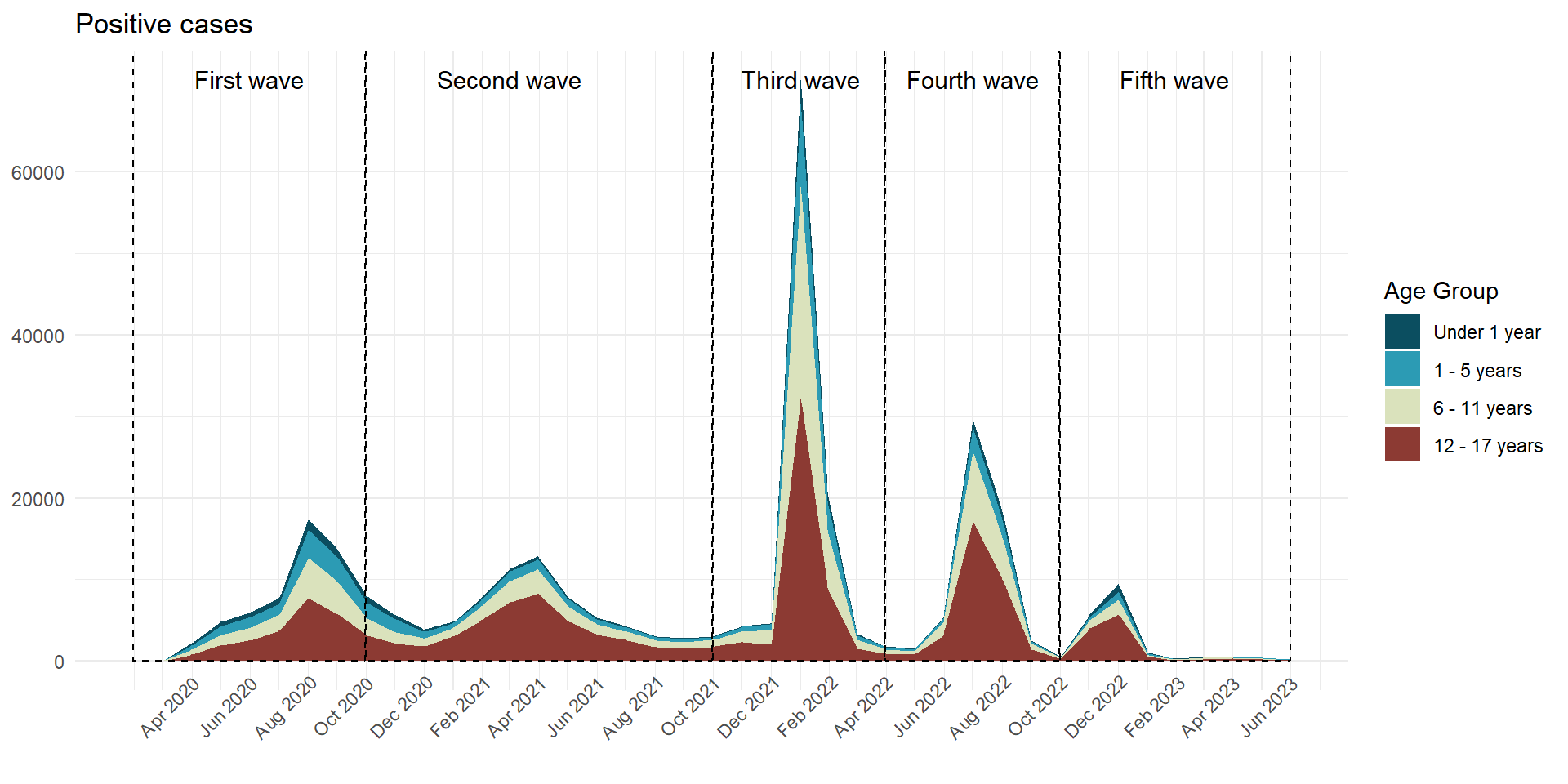
Gráfico de positivos (serie de tiempo) - Menores de 18 años

In [23]:

# 
# range_positivos_und_18 <- positivos %>% 
#   filter(edad < 18, 
#          sexo != "No registrado") %>% 
#   pull(fecha_resultado) %>%
#   range()

Sys.setlocale("LC_TIME", "English")

[1] "English_United States.1252"

positive_cases_area <- positivos_0723 %>% 
  mutate(
    fecha_round = case_when(
      fecha_round == as.Date("2024-01-01") ~  as.Date("2023-12-31"),
      .default = fecha_round
    )
  ) %>% 
  count(grupo_edad, fecha_round) %>% 
  collect() %>% 
  ggplot(
    aes(
      x = fecha_round,
      y = n,
      fill = grupo_edad
    )
  ) +
  geom_area(position = 'stack') +
  # innovar::scale_fill_innova("jama") +
  scale_fill_manual(
    values = c("#2C9BB4", "#0B4E60", "#DAE2BC", "#8C3A33")
  ) +
  scale_x_date(
    limits = c(ymd("2020-03-01"), ymd("2023-07-01")),
    breaks = seq(from = ceiling_date(ymd("2020-03-01"), "month"),
                 to = floor_date(ymd("2023-07-01"), "month"),
                 by = "2 months"), 
    # date_breaks = "2 month",
    date_labels = "%b %Y"
  ) +
  labs(
    y = NULL,
    x = NULL,
    title = "COVID-19 cases",
    fill = "Age Group"
  ) + 
  annotate(
    geom = "rect",
    xmin = as.Date("2020-03-01"), 
    xmax = as.Date("2020-10-31"), 
    ymin = 0, # El rectángulo se extiende hasta la parte inferior del gráfico
    ymax = Inf, # El rectángulo se extiende hasta la parte superior del gráfico
    color = "black", # Color de la línea
    fill = NA, # Sin relleno
    linetype = "dashed", # Tipo de línea discontinua
    linewidth = 0.5 # Grosor de la línea
  ) + 
  annotate(
    geom = "text", 
    x = as.Date("2020-07-01"), # Punto medio aproximado de la Ola 2
    y = Inf, # Posición vertical del texto
    label = "First wave", 
    color = "black",
    size = 4, # Tamaño del texto
    vjust = 2 # Ajuste vertical para colocar el texto encima del rectángulo
  ) +
  annotate(
    geom = "rect",
    xmin = as.Date("2020-11-01"), 
    xmax = as.Date("2021-10-31"), 
    ymin = 0, # El rectángulo se extiende hasta la parte inferior del gráfico
    ymax = Inf, # El rectángulo se extiende hasta la parte superior del gráfico
    color = "black", # Color de la línea
    fill = NA, # Sin relleno
    linetype = "dashed", # Tipo de línea discontinua
    linewidth = 0.5 # Grosor de la línea
  ) + 
  annotate(
    geom = "text", 
    x = as.Date("2021-05-10"), # Punto medio aproximado de la Ola 2
    y = Inf, # Posición vertical del texto
    label = "Second wave", 
    color = "black",
    size = 4, # Tamaño del texto
    vjust = 2 # Ajuste vertical para colocar el texto encima del rectángulo
  ) + 
  annotate(
    geom = "rect",
    xmin = as.Date("2021-11-01"), 
    xmax = as.Date("2022-04-30"), 
    ymin = 0, # El rectángulo se extiende hasta la parte inferior del gráfico
    ymax = Inf, # El rectángulo se extiende hasta la parte superior del gráfico
    color = "black", # Color de la línea
    fill = NA, # Sin relleno
    linetype = "dashed", # Tipo de línea discontinua
    linewidth = 0.5 # Grosor de la línea
  ) + 
    annotate(
    geom = "text", 
    x = as.Date("2022-02-01"), # Punto medio aproximado de la Ola 2
    y = Inf, # Posición vertical del texto
    label = "Third \nwave", 
    color = "black",
    size = 4, # Tamaño del texto
    vjust = 1.25 # Ajuste vertical para colocar el texto encima del rectángulo
  ) + 
  annotate(
    geom = "rect",
    xmin = as.Date("2022-05-01"), 
    xmax = as.Date("2022-10-31"), 
    ymin = 0, # El rectángulo se extiende hasta la parte inferior del gráfico
    ymax = Inf, # El rectángulo se extiende hasta la parte superior del gráfico
    color = "black", # Color de la línea
    fill = NA, # Sin relleno
    linetype = "dashed", # Tipo de línea discontinua
    linewidth = 0.5 # Grosor de la línea
  ) + 
  annotate(
    geom = "text", 
    x = as.Date("2022-08-01"), # Punto medio aproximado de la Ola 2
    y = Inf, # Posición vertical del texto
    label = "Fourth \nwave", 
    color = "black",
    size = 4, # Tamaño del texto
    vjust = 1.25 # Ajuste vertical para colocar el texto encima del rectángulo
  ) +
  annotate(
    geom = "rect",
    xmin = as.Date("2022-11-01"), 
    xmax = as.Date("2023-07-01"), 
    ymin = 0, # El rectángulo se extiende hasta la parte inferior del gráfico
    ymax = Inf, # El rectángulo se extiende hasta la parte superior del gráfico
    color = "black", # Color de la línea
    fill = NA, # Sin relleno
    linetype = "dashed", # Tipo de línea discontinua
    linewidth = 0.5 # Grosor de la línea
  ) + 
  annotate(
    geom = "text", 
    x = as.Date("2023-03-01"),
    y = Inf, # Posición vertical del texto
    label = "Fifth wave", 
    color = "black",
    size = 4, # Tamaño del texto
    vjust = 2 # Ajuste vertical para colocar el texto encima del rectángulo
  ) +
  theme_classic() +
  theme(
    axis.text.x = element_text(
      angle = 75,
      vjust = 0.5
    ),
    axis.ticks.x = element_line()
  ) 

positive_cases_area

Warning: Removed 4 rows containing non-finite outside the scale range
(`stat_align()`).

Figura 1: Positividad COVID Población menor de edad de acuerdo al grupo de edad y ola (07-03-2020 a 17-06-2023)

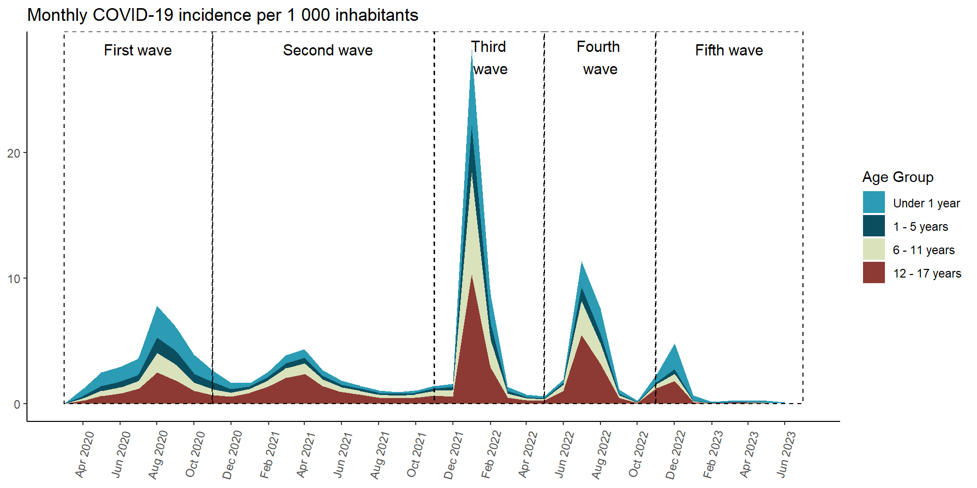
Gráfico de Incidencia (serie de tiempo) - Menores de 18 años

In [24]:

prevalence_by_age_area <- results_per_month_prevalencia$grupo_edad$index %>% 
  mutate(
    time = make_date(anio, mes, "1")
  ) %>% 
  ggplot(
    aes(
      x = time,
      y = rate,
      fill = grupo_edad
    )
  ) +
  geom_area(position = 'stack') +
  scale_fill_manual(
    values = c("#2C9BB4", "#0B4E60", "#DAE2BC", "#8C3A33")
  ) +
  scale_x_date(
    limits = c(ymd("2020-03-01"), ymd("2023-07-01")),
    breaks = seq(from = ceiling_date(ymd("2020-03-01"), "month"),
                 to = floor_date(ymd("2023-07-01"), "month"),
                 by = "2 months"), 
    # date_breaks = "2 month",
    date_labels = "%b %Y"
  ) +
  labs(
    y = NULL,
    x = NULL,
    title = "Monthly COVID-19 incidence per 1 000 inhabitants",
    fill = "Age Group"
  ) + 
  annotate(
    geom = "rect",
    xmin = as.Date("2020-03-01"), 
    xmax = as.Date("2020-10-31"), 
    ymin = 0, # El rectángulo se extiende hasta la parte inferior del gráfico
    ymax = Inf, # El rectángulo se extiende hasta la parte superior del gráfico
    color = "black", # Color de la línea
    fill = NA, # Sin relleno
    linetype = "dashed", # Tipo de línea discontinua
    linewidth = 0.5 # Grosor de la línea
  ) + 
  annotate(
    geom = "text", 
    x = as.Date("2020-07-01"), # Punto medio aproximado de la Ola 2
    y = Inf, # Posición vertical del texto
    label = "First wave", 
    color = "black",
    size = 4, # Tamaño del texto
    vjust = 2 # Ajuste vertical para colocar el texto encima del rectángulo
  ) +
  annotate(
    geom = "rect",
    xmin = as.Date("2020-11-01"), 
    xmax = as.Date("2021-10-31"), 
    ymin = 0, # El rectángulo se extiende hasta la parte inferior del gráfico
    ymax = Inf, # El rectángulo se extiende hasta la parte superior del gráfico
    color = "black", # Color de la línea
    fill = NA, # Sin relleno
    linetype = "dashed", # Tipo de línea discontinua
    linewidth = 0.5 # Grosor de la línea
  ) + 
  annotate(
    geom = "text", 
    x = as.Date("2021-05-10"), # Punto medio aproximado de la Ola 2
    y = Inf, # Posición vertical del texto
    label = "Second wave", 
    color = "black",
    size = 4, # Tamaño del texto
    vjust = 2 # Ajuste vertical para colocar el texto encima del rectángulo
  ) + 
  annotate(
    geom = "rect",
    xmin = as.Date("2021-11-01"), 
    xmax = as.Date("2022-04-30"), 
    ymin = 0, # El rectángulo se extiende hasta la parte inferior del gráfico
    ymax = Inf, # El rectángulo se extiende hasta la parte superior del gráfico
    color = "black", # Color de la línea
    fill = NA, # Sin relleno
    linetype = "dashed", # Tipo de línea discontinua
    linewidth = 0.5 # Grosor de la línea
  ) + 
  annotate(
    geom = "text", 
    x = as.Date("2022-02-01"), # Punto medio aproximado de la Ola 2
    y = Inf, # Posición vertical del texto
    label = "Third \nwave", 
    color = "black",
    size = 4, # Tamaño del texto
    vjust = 1.25 # Ajuste vertical para colocar el texto encima del rectángulo
  ) + 
  annotate(
    geom = "rect",
    xmin = as.Date("2022-05-01"), 
    xmax = as.Date("2022-10-31"), 
    ymin = 0, # El rectángulo se extiende hasta la parte inferior del gráfico
    ymax = Inf, # El rectángulo se extiende hasta la parte superior del gráfico
    color = "black", # Color de la línea
    fill = NA, # Sin relleno
    linetype = "dashed", # Tipo de línea discontinua
    linewidth = 0.5 # Grosor de la línea
  ) + 
  annotate(
    geom = "text", 
    x = as.Date("2022-08-01"), # Punto medio aproximado de la Ola 2
    y = Inf, # Posición vertical del texto
    label = "Fourth \nwave", 
    color = "black",
    size = 4, # Tamaño del texto
    vjust = 1.25 # Ajuste vertical para colocar el texto encima del rectángulo
  ) +
  annotate(
    geom = "rect",
    xmin = as.Date("2022-11-01"), 
    xmax = as.Date("2023-07-01"), 
    ymin = 0, # El rectángulo se extiende hasta la parte inferior del gráfico
    ymax = Inf, # El rectángulo se extiende hasta la parte superior del gráfico
    color = "black", # Color de la línea
    fill = NA, # Sin relleno
    linetype = "dashed", # Tipo de línea discontinua
    linewidth = 0.5 # Grosor de la línea
  ) + 
  annotate(
    geom = "text", 
    x = as.Date("2023-03-01"),
    y = Inf, # Posición vertical del texto
    label = "Fifth wave", 
    color = "black",
    size = 4, # Tamaño del texto
    vjust = 2 # Ajuste vertical para colocar el texto encima del rectángulo
  ) +
  theme_classic() +
  theme(
    axis.text.x = element_text(
      angle = 75,
      vjust = 0.5
    ),
    axis.ticks.x = element_line()
  ) 

prevalence_by_age_area

Warning: Removed 4 rows containing non-finite outside the scale range
(`stat_align()`).

Figura 2: Incidencia COVID Población menor de edad de acuerdo al grupo de edad y ola (07-03-2020 a 17-06-2023)

Pirámide frecuencia - Edades

In [25]:

positivos_0723_tbl %>% 
  mutate(
    edad = factor(edad)
  ) %>% 
  age_pyramid(
    age_group = "edad",
    split_by = "sexo"
  ) +
  scale_fill_brewer(palette = "Dark2") +
  labs(
    x = "Age",
    fill = "Sex",
    y = "Frequency"
  ) +
  theme_classic()

Scale for fill is already present.
Adding another scale for fill, which will replace the existing scale.

In [26]:

positivos_0723_tbl %>% 
  age_pyramid(
    age_group = "grupo_edad",
    split_by = "sexo"
  ) +
  scale_fill_brewer(palette = "Dark2") +
  labs(
    x = "Age Group",
    fill = "Sex",
    y = "Frequency"
  ) +
  scale_y_continuous(
    labels = ~ scales::number(abs(.x), big.mark = ","),
    n.breaks = 10
  ) +
  theme_classic()

Scale for fill is already present.
Adding another scale for fill, which will replace the existing scale.
Scale for y is already present.
Adding another scale for y, which will replace the existing scale.

Pirámide proporcional - Edades

In [27]:

positivos_0723_tbl %>% 
  mutate(
    edad = factor(edad)
  ) %>% 
  age_pyramid(
    age_group = "edad",
    split_by = "sexo",
    proportional = TRUE
  ) +
   scale_fill_brewer(palette = "Dark2") +
  labs(
    x = "Age",
    fill = "Sex",
    y = "Percentage"
  ) +
  theme_classic()

Scale for fill is already present.
Adding another scale for fill, which will replace the existing scale.

In [28]:

positivos_0723_tbl %>% 
  age_pyramid(
    age_group = "grupo_edad",
    split_by = "sexo",
    proportional = TRUE
  ) +
   scale_fill_brewer(palette = "Dark2") +
  labs(
    x = "Age Group",
    fill = "Sex",
    y = "Percentage"
  ) +
  theme_classic()

Scale for fill is already present.
Adding another scale for fill, which will replace the existing scale.

Departamento

In [29]:

prev_dep_1k_sf <- peru_dep_sf %>% 
  rename(departamento = dep) %>% 
  inner_join(
    results_prevalencia$departamento$index
  )

Joining with `by = join_by(departamento)`

In [30]:

prev_dep_1k_map <- prev_dep_1k_sf %>%
  ggplot() +
  geom_sf(aes(fill = rate)) +
  guides(
    fill = guide_legend(
      str_wrap("Mean monthly COVID-19 incidence", 
               20)
    )
  ) +
  scale_fill_distiller(palette = "Oranges", # old: YlOrBr
                       direction = 1,
                       guide = "legend") + 
  theme_void()

prev_dep_1k_map

Figura 3: Prevalencia COVID-19 de acuerdo al departamento (07-03-2020 a 17-06-2023)

In [31]:

In [32]:

tbl_summ_prev_dep_pre <- results_prevalencia$departamento$index %>% 
  mutate(
    rate = formattable::digits(rate, 3)
  ) %>% 
  mutate(
    departamento = str_to_title(departamento)
  ) 

tbl_summ_prev_dep <- tbl_summ_prev_dep_pre %>% 
  rename_with(
    .fn = ~ paste0("**", str_to_title(.x), "**")
  ) %>% 
  gt::gt() %>% 
  gt::cols_label(
    .fn = gt::md,
    .process_units = TRUE
  )

tbl_summ_prev_dep

Tabla 4: Prevalencia COVID-19 de acuerdo al departamento (07-03-2020 a 17-06-2023)

Departamento	Rate
Amazonas	0.802
Ancash	0.903
Apurimac	0.587
Arequipa	1.264
Ayacucho	0.394
Cajamarca	0.452
Callao	0.782
Cusco	0.518
Huancavelica	0.466
Huanuco	0.430
Ica	1.085
Junin	0.740
La Libertad	0.520
Lambayeque	0.517
Lima	1.232
Loreto	0.459
Madre De Dios	1.333
Moquegua	2.615
Pasco	0.719
Piura	0.670
Puno	0.337
San Martin	0.657
Tacna	1.416
Tumbes	1.215
Ucayali	0.620

In [33]:

tbl_summ_prev_dep_pre %>% 
  rename_with(
    .fn = str_to_title
  ) %>% 
  huxtable::as_hux() %>% 
  huxtable::set_bold(1, 1:2) %>% 
  huxtable::quick_xlsx(file = "02_output/tables/prevalencia_departamento.xlsx",
                       open = FALSE)

tbl_summ_prev_dep %>%
  gt::gtsave("02_output/tables/prevalencia_departamento.docx")

In [34]:

downloadthis::download_file(
  path = "02_output/tables/prevalencia_departamento.xlsx",
  button_label = "Descargar tabla en Excel",
  button_type = "success",
  has_icon = TRUE,
  icon = "fa fa-save"
)

In [35]:

downloadthis::download_file(
  path = "02_output/tables/prevalencia_departamento.docx",
  button_label = "Descargar tabla en Word",
  button_type = "primary",
  has_icon = TRUE,
  icon = "fa fa-save"
)

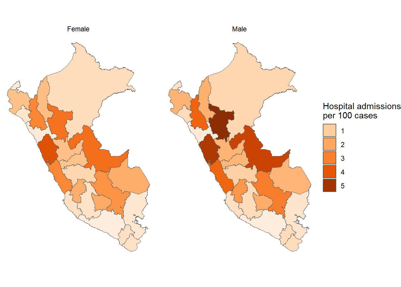
Departamento y sexo

In [36]:

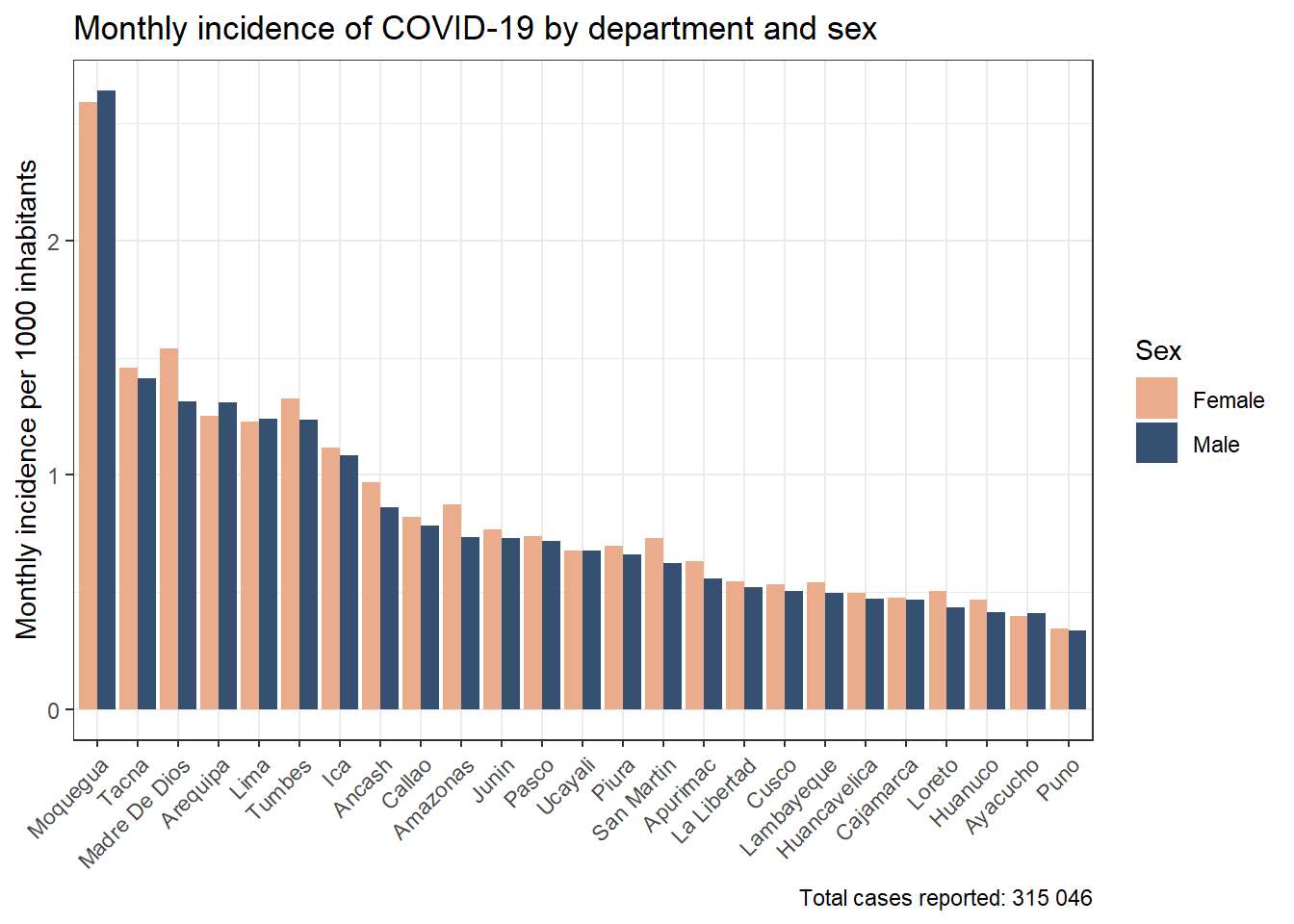
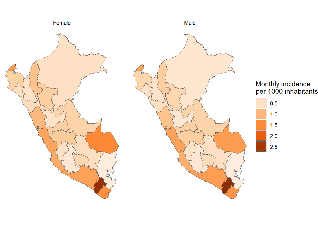
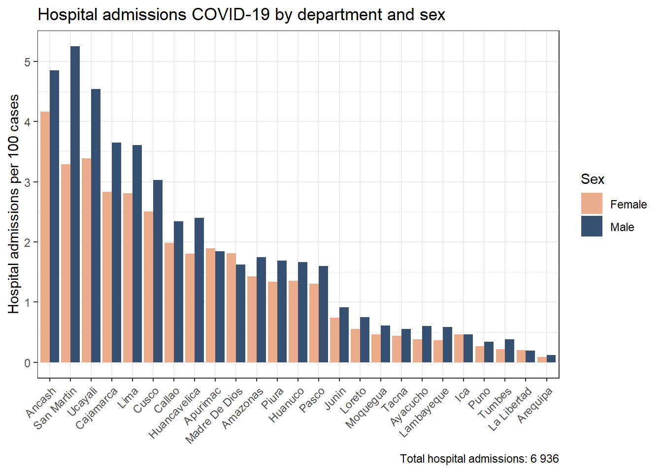
results_prevalencia$departamento_sexo$index %>% 
  mutate(
    departamento = str_to_title(departamento),
    departamento = fct_reorder2(departamento, sexo, rate)
  ) %>% 
  ggplot(aes(x = departamento, y = rate, fill = sexo)) +
  geom_bar(stat = "identity", position = position_dodge()) +
  theme_bw() +
  labs(title = "Monthly incidence of COVID-19 by department and sex", 
       x = NULL, 
       y = "Mean monthly COVID-19 incidence",
       fill = "Sex",
       caption = paste0("Total cases reported: ", 
                        scales::number(sum(pull(results_prevalencia$departamento_sexo$index_pre,
                                                count))))) +
  innovar::scale_fill_innova("blue_fall") +
  theme(
    axis.text.x = element_text(
      angle = 45,
      hjust = 1,
      vjust = 1
    )
  )

Figura 4: Prevalencia COVID-19 de acuerdo al departamento y sexo (07-03-2020 a 17-06-2023)

In [37]:

prev_dep_sex_1k_sf <- peru_dep_sf %>% 
  rename(departamento = dep) %>% 
  inner_join(
    results_prevalencia$departamento_sexo$index
  ) %>% 
  ungroup()

Joining with `by = join_by(departamento)`

In [38]:

prev_dep_sex_1k_sf %>%
  ggplot() +
  geom_sf(aes(fill = rate)) +
  guides(
    fill = guide_legend(
      str_wrap(
        "Mean monthly COVID-19 incidence",
        20
      )
    )
  ) +
  scale_fill_distiller(palette = "Oranges", # old: YlOrBr
                       direction = 1) + 
  facet_wrap(vars(sexo)) + 
  theme_void()

Figura 5: Prevalencia COVID-19 de acuerdo al departamento y sexo (07-03-2020 a 17-06-2023)

In [39]:

In [40]:

tbl_summ_prev_dep_sex_pre <- results_prevalencia$departamento_sexo$index %>% 
  mutate(
    rate = formattable::digits(rate, 3),
    departamento = str_to_title(departamento)
  ) %>% 
  pivot_wider(
    names_from = sexo, 
    values_from = rate
  )

tbl_summ_prev_dep_sex <- tbl_summ_prev_dep_sex_pre %>% 
  rename_with(
    .fn = ~ paste0("**", str_to_title(.x), "**")
  ) %>% 
  gt::gt() %>% 
  gt::cols_label(
    .fn = gt::md,
    .process_units = TRUE
  )

tbl_summ_prev_dep_sex

Tabla 5: Prevalencia COVID-19 de acuerdo al departamento y sexo (07-03-2020 a 17-06-2023)

Departamento	Female	Male
Amazonas	0.874	0.733
Ancash	0.969	0.862
Apurimac	0.630	0.559
Arequipa	1.252	1.308
Ayacucho	0.399	0.411
Cajamarca	0.475	0.466
Callao	0.820	0.785
Cusco	0.533	0.504
Huancavelica	0.498	0.473
Huanuco	0.469	0.414
Ica	1.115	1.083
Junin	0.768	0.731
La Libertad	0.545	0.522
Lambayeque	0.540	0.495
Lima	1.227	1.238
Loreto	0.505	0.436
Madre De Dios	1.538	1.313
Moquegua	2.590	2.641
Pasco	0.740	0.717
Piura	0.699	0.659
Puno	0.346	0.338
San Martin	0.730	0.623
Tacna	1.456	1.414
Tumbes	1.325	1.237
Ucayali	0.677	0.676

In [41]:

tbl_summ_prev_dep_sex_pre %>% 
  rename_with(
    .fn = str_to_title
  ) %>% 
  huxtable::as_hux() %>% 
  huxtable::set_bold(1, 1:3) %>% 
  huxtable::quick_xlsx(file = "02_output/tables/prevalencia_departamento_sexo.xlsx",
                       open = FALSE)

tbl_summ_prev_dep_sex %>%
  gt::gtsave("02_output/tables/prevalencia_departamento_sexo.docx")

In [42]:

downloadthis::download_file(
  path = "02_output/tables/prevalencia_departamento_sexo.xlsx",
  button_label = "Descargar tabla en Excel",
  button_type = "success",
  has_icon = TRUE,
  icon = "fa fa-save"
)

In [43]:

downloadthis::download_file(
  path = "02_output/tables/prevalencia_departamento_sexo.docx",
  button_label = "Descargar tabla en Word",
  button_type = "primary",
  has_icon = TRUE,
  icon = "fa fa-save"
)

Departamento y edad

In [44]:

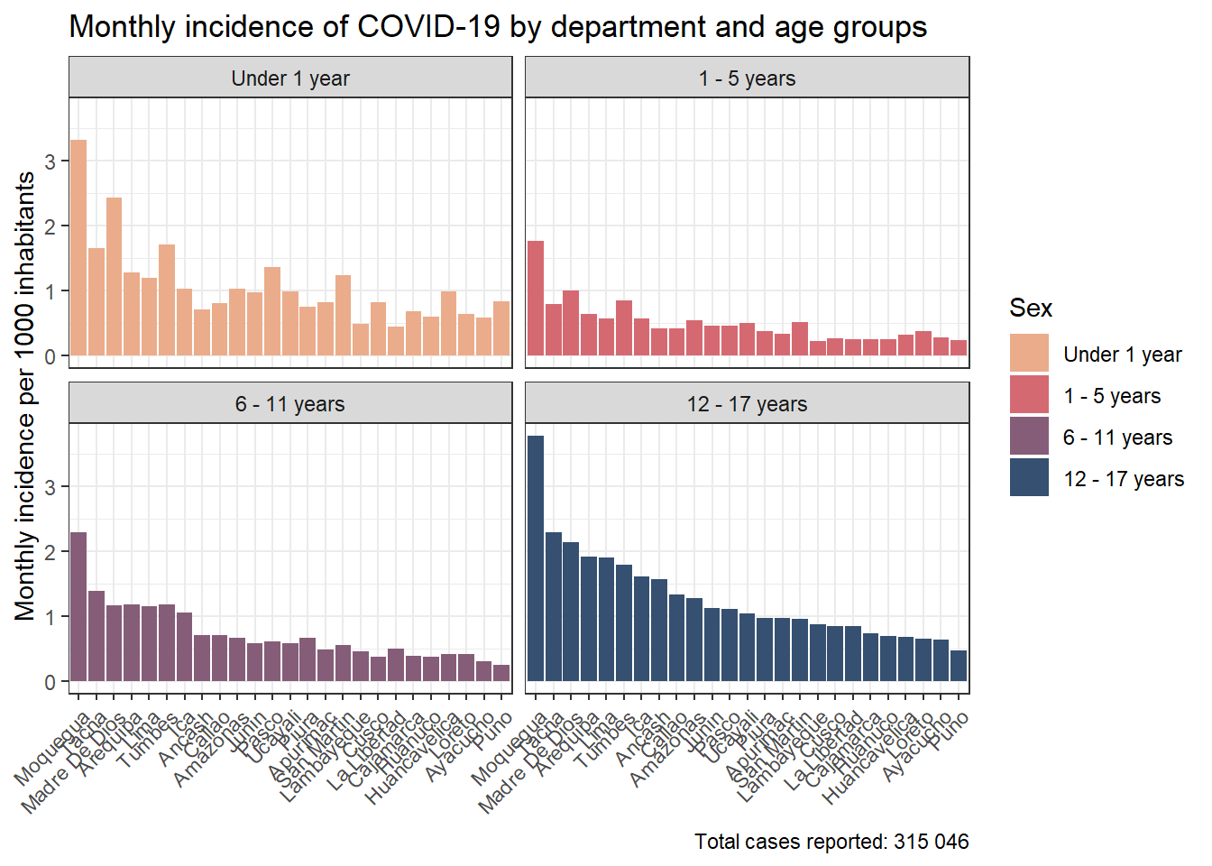
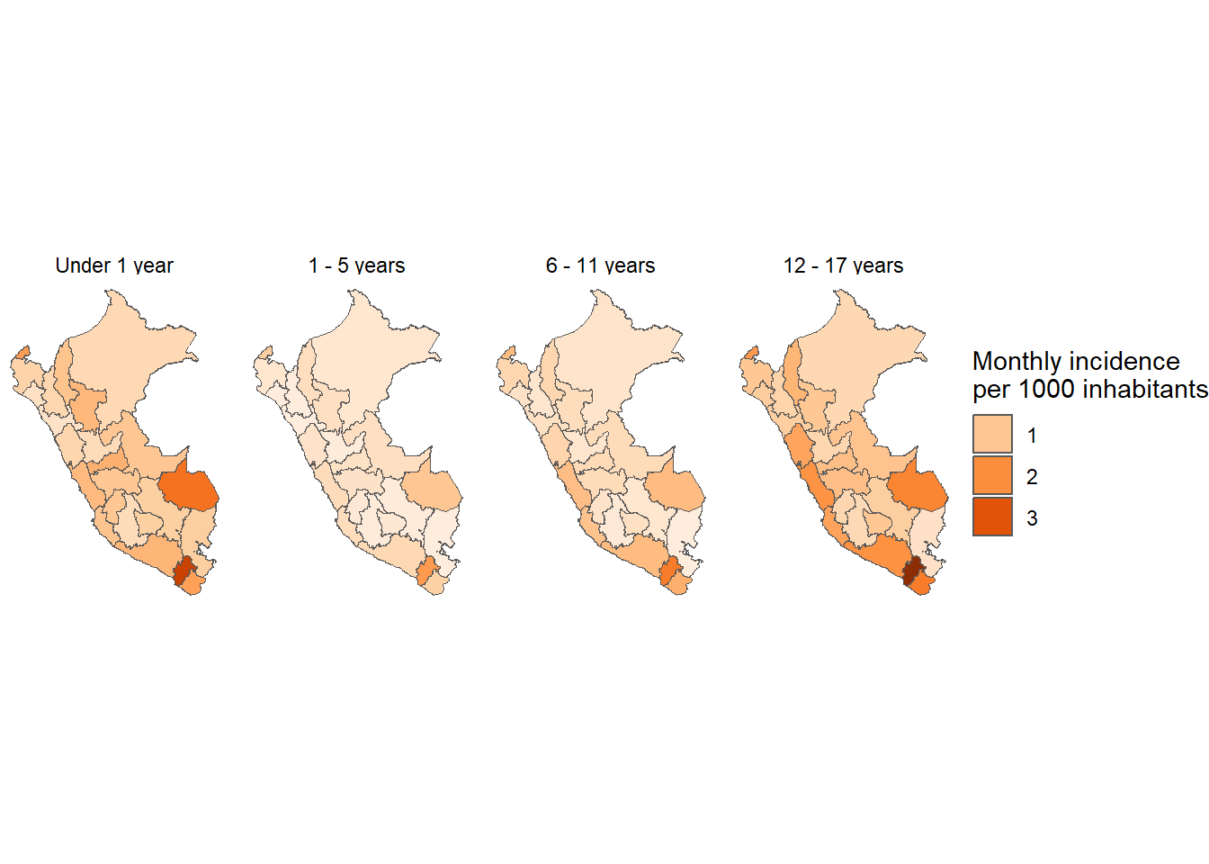
results_prevalencia$departamento_grupo_edad$index %>% 
  mutate(
    departamento = str_to_title(departamento),
    departamento = fct_reorder2(departamento, grupo_edad, rate)
  ) %>% 
  ggplot(aes(x = departamento, y = rate, fill = grupo_edad)) +
  geom_bar(stat = "identity") +
  theme_bw() +
  labs(title = "Monthly incidence of COVID-19 by department and age groups", 
       x = NULL, 
       y = "Mean monthly COVID-19 incidence",
       fill = "Sex",
       caption = paste0("Total cases reported: ", 
                        scales::number(sum(pull(results_prevalencia$departamento_grupo_edad$index_pre,
                                                count))))) +
  innovar::scale_fill_innova("blue_fall") +
  facet_wrap(vars(grupo_edad)) + 
  theme(
    axis.text.x = element_text(
      angle = 45,
      hjust = 1,
      vjust = 1
    )
  )

Figura 6: Prevalencia COVID-19 de acuerdo al departamento y edad (07-03-2020 a 17-06-2023)

In [45]:

prev_dep_edad_1k_sf <- peru_dep_sf %>% 
  rename(departamento = dep) %>% 
  inner_join(
    results_prevalencia$departamento_grupo_edad$index
  ) %>% 
  ungroup()

Joining with `by = join_by(departamento)`

In [46]:

prev_dep_edad_1k_sf %>%
  ggplot() +
  geom_sf(aes(fill = rate)) +
  guides(
    fill = guide_legend(
      str_wrap(
        "Mean monthly COVID-19 incidence",
        20
      )
    )
  ) +
  scale_fill_distiller(palette = "Oranges", # old: YlOrBr
                       direction = 1) + 
  facet_wrap(vars(grupo_edad), nrow = 1) + 
  theme_void()

Figura 7: Prevalencia COVID-19 de acuerdo al departamento y edad (07-03-2020 a 17-06-2023)

In [47]:

In [48]:

tbl_summ_prev_dep_edad_pre <- results_prevalencia$departamento_grupo_edad$index %>% 
  mutate(
    rate = formattable::digits(rate, 3)
  ) %>% 
  mutate(
    departamento = str_to_title(departamento)
  ) %>% 
  pivot_wider(
    names_from = grupo_edad, 
    values_from = rate
  )

tbl_summ_prev_dep_edad <- tbl_summ_prev_dep_edad_pre %>% 
  rename_with(
    .fn = ~ paste0("**", str_to_title(.x), "**")
  ) %>% 
  gt::gt() %>% 
  gt::cols_label(
    .fn = gt::md,
    .process_units = TRUE
  )

tbl_summ_prev_dep_edad

Tabla 6: Prevalencia COVID-19 de acuerdo al departamento y grupo de edad (07-03-2020 a 17-06-2023)

Departamento	Under 1 Year	1 - 5 Years	6 - 11 Years	12 - 17 Years
Amazonas	1.038	0.546	0.677	1.283
Ancash	0.710	0.428	0.719	1.579
Apurimac	0.824	0.341	0.493	0.977
Arequipa	1.278	0.645	1.179	1.922
Ayacucho	0.583	0.283	0.312	0.638
Cajamarca	0.683	0.254	0.387	0.743
Callao	0.806	0.426	0.720	1.340
Cusco	0.830	0.267	0.377	0.855
Huancavelica	0.988	0.323	0.425	0.687
Huanuco	0.597	0.258	0.386	0.698
Ica	1.032	0.569	1.055	1.613
Junin	0.978	0.459	0.592	1.132
La Libertad	0.450	0.253	0.503	0.853
Lambayeque	0.487	0.232	0.469	0.876
Lima	1.200	0.578	1.151	1.902
Loreto	0.646	0.378	0.417	0.651
Madre De Dios	2.436	0.999	1.172	2.149
Moquegua	3.323	1.774	2.294	3.788
Pasco	1.362	0.465	0.616	1.121
Piura	0.759	0.376	0.676	0.982
Puno	0.844	0.248	0.253	0.470
San Martin	1.240	0.521	0.555	0.967
Tacna	1.664	0.793	1.389	2.292
Tumbes	1.712	0.857	1.179	1.800
Ucayali	0.994	0.507	0.588	1.043

In [49]:

tbl_summ_prev_dep_edad_pre %>% 
  rename_with(
    .fn = str_to_title
  ) %>% 
  huxtable::as_hux() %>% 
  huxtable::set_bold(1, 1:5) %>% 
  huxtable::quick_xlsx(file = "02_output/tables/prevalencia_departamento_edad.xlsx",
                       open = FALSE)

tbl_summ_prev_dep_edad %>%
  gt::gtsave("02_output/tables/prevalencia_departamento_edad.docx")

In [50]:

downloadthis::download_file(
  path = "02_output/tables/prevalencia_departamento_edad.xlsx",
  button_label = "Descargar tabla en Excel",
  button_type = "success",
  has_icon = TRUE,
  icon = "fa fa-save"
)

In [51]:

downloadthis::download_file(
  path = "02_output/tables/prevalencia_departamento_edad.docx",
  button_label = "Descargar tabla en Word",
  button_type = "primary",
  has_icon = TRUE,
  icon = "fa fa-save"
)

Departamento, sexo y grupo de edad

In [52]:

In [53]:

tbl_summ_prev_dep_edad_sex_pre <- results_prevalencia$departamento_sexo_grupo_edad$index %>% 
  mutate(
    rate = formattable::digits(rate, 3)
  ) %>% 
  pivot_wider(
    names_from = grupo_edad, 
    values_from = rate
  ) %>% 
  arrange(departamento, sexo) %>% 
  collect() %>% 
  mutate(
    departamento = str_to_title(departamento)
  ) 


tbl_summ_prev_dep_edad_sex <- tbl_summ_prev_dep_edad_sex_pre %>% 
  rename_with(
    .fn = ~ paste0("**", str_to_title(.x), "**")
  ) %>% 
  gt::gt() %>% 
  gt::cols_label(
    .fn = gt::md,
    .process_units = TRUE
  )
  # gt::cols_label(
  #   departamento = gt::md("**Departamento**"),
  #   sexo = gt::md("**Sexo**")
  # ) 
  # gt::tab_style(
  #   style = gt::cell_text(weight = "bold"),
  #   locations = gt::cells_column_labels()
  # )

tbl_summ_prev_dep_edad_sex

Tabla 7: Prevalencia COVID-19 de acuerdo al departamento, edad y sexo (07-03-2020 a 17-06-2023)

Departamento	Sexo	Under 1 Year	1 - 5 Years	6 - 11 Years	12 - 17 Years
Amazonas	Female	1.250	0.569	0.729	1.564
Amazonas	Male	1.194	0.576	0.748	1.079
Ancash	Female	0.815	0.445	0.702	1.768
Ancash	Male	0.791	0.434	0.736	1.433
Apurimac	Female	0.930	0.382	0.529	1.159
Apurimac	Male	0.917	0.384	0.593	0.882
Arequipa	Female	1.304	0.625	1.127	1.981
Arequipa	Male	1.506	0.664	1.294	1.910
Ayacucho	Female	0.692	0.284	0.310	0.761
Ayacucho	Male	0.733	0.336	0.342	0.592
Cajamarca	Female	0.687	0.256	0.396	0.849
Cajamarca	Male	0.784	0.268	0.413	0.699
Callao	Female	0.866	0.442	0.785	1.444
Callao	Male	1.012	0.462	0.740	1.345
Cusco	Female	0.760	0.251	0.367	0.945
Cusco	Male	0.971	0.297	0.397	0.788
Huancavelica	Female	1.042	0.375	0.429	0.768
Huancavelica	Male	1.333	0.337	0.474	0.670
Huanuco	Female	0.663	0.280	0.439	0.789
Huanuco	Male	0.708	0.293	0.396	0.683
Ica	Female	1.188	0.567	1.055	1.770
Ica	Male	1.367	0.587	1.085	1.544
Junin	Female	0.892	0.440	0.626	1.215
Junin	Male	1.087	0.527	0.604	1.051
La Libertad	Female	0.453	0.250	0.507	0.933
La Libertad	Male	0.597	0.293	0.526	0.836
Lambayeque	Female	0.515	0.232	0.467	0.992
Lambayeque	Male	0.578	0.238	0.498	0.784
Lima	Female	1.082	0.561	1.103	1.951
Lima	Male	1.342	0.594	1.201	1.851
Loreto	Female	0.732	0.475	0.477	0.800
Loreto	Male	0.730	0.365	0.452	0.555
Madre De Dios	Female	3.025	1.034	1.290	2.701
Madre De Dios	Male	2.887	1.277	1.307	1.968
Moquegua	Female	3.841	1.847	2.453	3.933
Moquegua	Male	4.528	2.089	2.461	3.956
Pasco	Female	1.714	0.487	0.626	1.255
Pasco	Male	1.780	0.533	0.696	1.046
Piura	Female	0.812	0.356	0.639	1.104
Piura	Male	0.836	0.407	0.714	0.912
Puno	Female	0.800	0.234	0.247	0.538
Puno	Male	1.021	0.277	0.288	0.453
San Martin	Female	1.265	0.555	0.554	1.200
San Martin	Male	1.390	0.544	0.592	0.798
Tacna	Female	1.885	0.784	1.567	2.435
Tacna	Male	2.039	0.929	1.473	2.215
Tumbes	Female	2.039	0.847	1.317	2.098
Tumbes	Male	2.218	1.002	1.244	1.674
Ucayali	Female	1.036	0.603	0.600	1.213
Ucayali	Male	1.211	0.518	0.678	1.005

In [54]:

tbl_summ_prev_dep_edad_sex_pre %>% 
  rename_with(
    .fn = str_to_title
  ) %>% 
  huxtable::as_hux() %>% 
  huxtable::set_bold(1, 1:6) %>% 
  huxtable::quick_xlsx(file = "02_output/tables/prevalencia_departamento_edad_sexo.xlsx",
                       open = FALSE)

tbl_summ_prev_dep_edad_sex %>%
  gt::gtsave("02_output/tables/prevalencia_departamento_edad_sexo.docx")

In [55]:

downloadthis::download_file(
  path = "02_output/tables/prevalencia_departamento_edad_sexo.xlsx",
  button_label = "Descargar tabla en Excel",
  button_type = "success",
  has_icon = TRUE,
  icon = "fa fa-save"
)

In [56]:

downloadthis::download_file(
  path = "02_output/tables/prevalencia_departamento_edad_sexo.docx",
  button_label = "Descargar tabla en Word",
  button_type = "primary",
  has_icon = TRUE,
  icon = "fa fa-save"
)

In [57]:

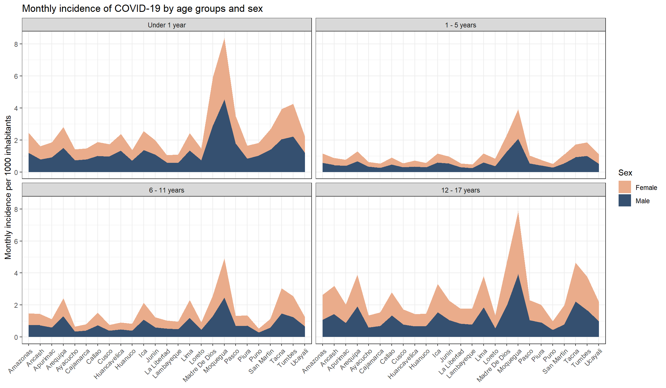
results_prevalencia$departamento_sexo_grupo_edad$index %>% 
  mutate(
    departamento = str_to_title(departamento)
  ) %>% 
  ggplot(
    aes(
      x = departamento,
      y = rate,
      fill = sexo,
      group = sexo
    )
  ) +
  geom_area() +
  facet_wrap(vars(grupo_edad)) +
  innovar::scale_fill_innova("blue_fall") +
  labs(
    y = "Mean monthly COVID-19 incidence",
    x = NULL,
    title = "Monthly incidence of COVID-19 by age groups and sex",
    fill = "Sex"
  ) + 
  theme_bw() +
  theme(
    axis.text.x = element_text(
      angle = 45,
      hjust = 1,
      vjust = 1
    )
  )

Figura 8: Prevalencia COVID-19 de acuerdo al departamento, sexo y edad (07-03-2020 a 17-06-2023)

Departamento y olas

In [58]:

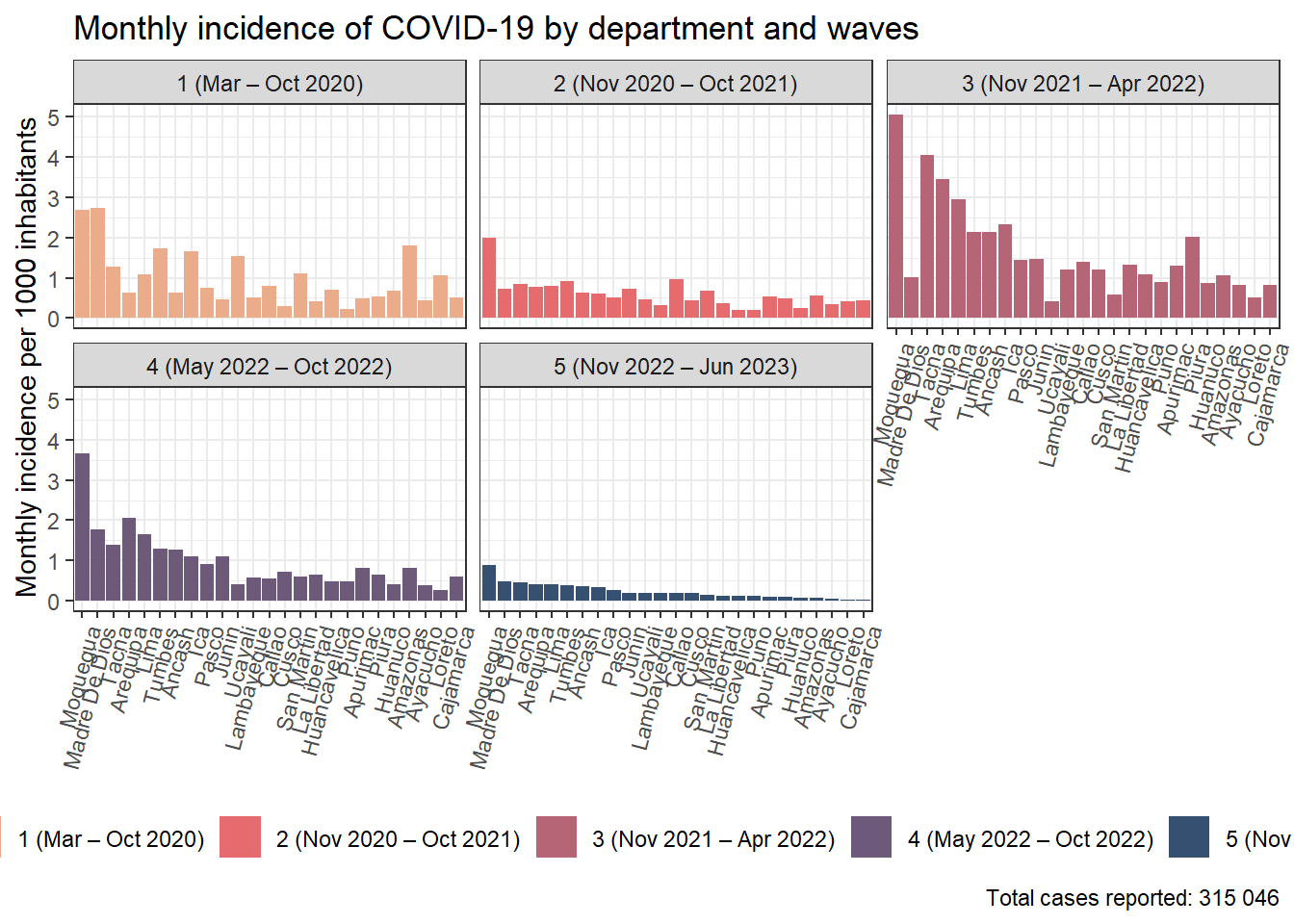
results_prevalencia$departamento_ola_covid$index %>% 
  drop_na(ola_covid) %>% 
  mutate(
    departamento = str_to_title(departamento),
    departamento = fct_reorder2(departamento, ola_covid, rate)
  ) %>% 
  ggplot(aes(x = departamento, y = rate, fill = ola_covid)) +
  geom_bar(stat = "identity") +
  theme_bw() +
  labs(title = "Monthly incidence of COVID-19 by department and waves", 
       x = NULL, 
       y = "Mean monthly COVID-19 incidence",
       fill = "Sexo",
       caption = paste0("Total cases reported: ", 
                        scales::number(sum(pull(results_prevalencia$departamento_ola_covid$index_pre,
                                                count))))) +
  innovar::scale_fill_innova("blue_fall") +
  facet_wrap(vars(ola_covid)) + 
  theme(
    axis.text.x = element_text(
      angle = 75,
      hjust = 1,
      vjust = 1
    ),
    legend.position = "bottom"
  )

Figura 9: Prevalencia COVID-19 de acuerdo al departamento y olas covid (07-03-2020 a 17-06-2023)

In [59]:

prev_dep_olas_100k <- results_prevalencia$departamento_ola_covid$index %>% 
  drop_na(ola_covid) %>% 
  bind_rows(
    results_prevalencia$departamento$index %>% 
      mutate(ola_covid = "Overall")
  ) %>% 
  mutate(
    ola_covid = fct_recode(
      ola_covid,
      "1st wave" = "1 (Mar – Oct 2020)",
      "2nd wave" = "2 (Nov 2020 – Oct 2021)",
      "3rd wave" = "3 (Nov 2021 – Apr 2022)",
      "4th wave" = "4 (May 2022 – Oct 2022)",
      "5th wave" = "5 (Nov 2022 – Jun 2023)"
    ),
    ola_covid = fct_relevel(ola_covid,
                            "Overall")
  ) %>% 
  arrange(ola_covid)


prev_mes_dep_olas_1k_sf <- peru_dep_sf %>%
  rename(departamento = dep) %>% 
  left_join(
    prev_dep_olas_100k
  ) %>%
  ungroup()

Joining with `by = join_by(departamento)`

In [60]:

prev_mes_dep_olas_1k_map <- prev_mes_dep_olas_1k_sf %>%
  ggplot() +
  geom_sf(aes(fill = rate)) +
  guides(
    fill = guide_legend(str_wrap("Mean monthly COVID-19 incidence", 20))
  ) +
  scale_fill_distiller(palette = "Oranges", # Old: YlOrBr
                       direction = 1) + 
  facet_wrap(vars(ola_covid), nrow = 1) + 
  theme_void()

prev_mes_dep_olas_1k_map

Figura 10: Prevalencia COVID-19 de acuerdo al departamento por Olas (07-03-2020 a 17-06-2023)

In [61]:

In [62]:

tbl_summ_prev_dep_ola_pre <- results_prevalencia$departamento_ola_covid$index %>% 
  drop_na(ola_covid) %>% 
  mutate(
    rate = formattable::digits(rate, 3)
  ) %>% 
  mutate(
    departamento = str_to_title(departamento)
  ) %>% 
  pivot_wider(
    names_from = ola_covid, 
    values_from = rate
  )

tbl_summ_prev_dep_ola <- tbl_summ_prev_dep_ola_pre %>% 
  rename_with(
    .fn = ~ paste0("**", str_to_title(.x), "**")
  ) %>% 
  gt::gt() %>% 
  gt::cols_label(
    .fn = gt::md,
    .process_units = TRUE
  )

tbl_summ_prev_dep_ola

Tabla 8: Prevalencia COVID-19 de acuerdo al departamento y Olas COVID (07-03-2020 a 17-06-2023)

Departamento	1 (Mar – Oct 2020)	2 (Nov 2020 – Oct 2021)	3 (Nov 2021 – Apr 2022)	4 (May 2022 – Oct 2022)	5 (Nov 2022 – Jun 2023)
Amazonas	1.800	0.565	1.067	0.812	0.079
Ancash	0.640	0.636	2.125	1.280	0.365
Apurimac	0.492	0.532	1.290	0.825	0.106
Arequipa	0.627	0.773	3.446	2.049	0.412
Ayacucho	0.445	0.349	0.816	0.387	0.061
Cajamarca	0.513	0.431	0.820	0.608	0.037
Callao	0.798	0.966	1.404	0.562	0.190
Cusco	0.285	0.429	1.201	0.728	0.187
Huancavelica	0.710	0.201	1.072	0.496	0.132
Huanuco	0.684	0.248	0.875	0.411	0.087
Ica	1.653	0.615	2.331	1.113	0.335
Junin	0.467	0.735	1.461	1.109	0.202
La Libertad	0.418	0.378	1.321	0.647	0.139
Lambayeque	0.520	0.323	1.214	0.582	0.195
Lima	1.082	0.809	2.943	1.662	0.412
Loreto	1.057	0.405	0.515	0.267	0.043
Madre De Dios	2.737	0.732	1.022	1.772	0.494
Moquegua	2.671	1.996	5.052	3.654	0.887
Pasco	0.751	0.513	1.435	0.915	0.259
Piura	0.547	0.480	2.006	0.643	0.098
Puno	0.219	0.199	0.893	0.488	0.119
San Martin	1.104	0.669	0.583	0.600	0.146
Tacna	1.267	0.841	4.048	1.382	0.460
Tumbes	1.724	0.920	2.141	1.300	0.389
Ucayali	1.546	0.458	0.411	0.423	0.199

In [63]:

tbl_summ_prev_dep_ola_pre %>% 
  rename_with(
    .fn = str_to_title
  ) %>% 
  huxtable::as_hux() %>% 
  huxtable::set_bold(1, 1:6) %>% 
  huxtable::quick_xlsx(file = "02_output/tables/prevalencia_departamento_ola.xlsx",
                       open = FALSE)

tbl_summ_prev_dep_ola %>%
  gt::gtsave("02_output/tables/prevalencia_departamento_ola.docx")

In [64]:

downloadthis::download_file(
  path = "02_output/tables/prevalencia_departamento_ola.xlsx",
  button_label = "Descargar tabla en Excel",
  button_type = "success",
  has_icon = TRUE,
  icon = "fa fa-save"
)

In [65]:

downloadthis::download_file(
  path = "02_output/tables/prevalencia_departamento_ola.docx",
  button_label = "Descargar tabla en Word",
  button_type = "primary",
  has_icon = TRUE,
  icon = "fa fa-save"
)

Regiones

In [66]:

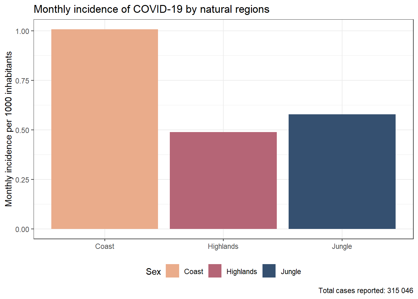
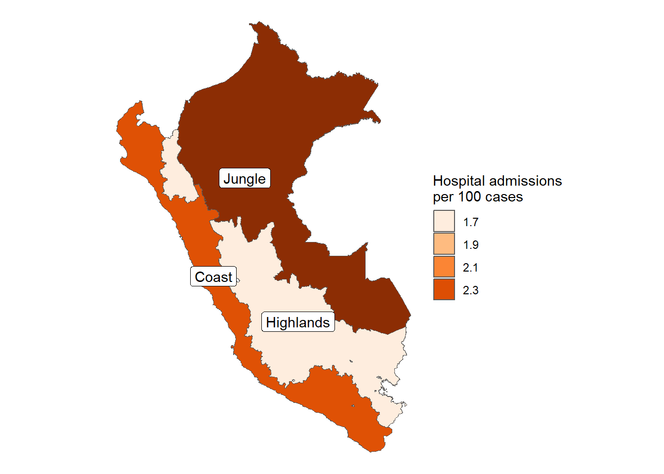
results_prevalencia$region$index %>% 
  ggplot(aes(x = region, y = rate, fill = region)) +
  geom_bar(stat = "identity") +
  theme_bw() +
  labs(title = "Monthly incidence of COVID-19 by natural regions", 
       x = NULL, 
       y = "Mean monthly COVID-19 incidence",
       fill = "Sex",
       caption = paste0("Total cases reported: ", 
                        scales::number(sum(pull(results_prevalencia$region$index_pre,
                                                count))))) +
  innovar::scale_fill_innova("blue_fall") +
  theme(
    legend.position = "bottom"
  )

Figura 11: Prevalencia COVID-19 de acuerdo a la región (07-03-2020 a 17-06-2023)

In [67]:

prev_reg_1k_sf <- peru_reg_sf %>% 
  inner_join(
    results_prevalencia$region$index
  )

Joining with `by = join_by(region)`

In [68]:

prev_reg_1k_map <- prev_reg_1k_sf %>%
  ggplot() +
  geom_sf(aes(fill = rate)) +
  guides(
    fill = guide_legend(
      str_wrap("Mean monthly COVID-19 incidence", 
               20)
    )
  ) +
  ggsflabel::geom_sf_label(aes(label = region)) +
  scale_fill_distiller(palette = "Oranges", # YlOrBr
                       direction = 1) + 
  theme_void()

prev_reg_1k_map

Warning in st_point_on_surface.sfc(data$geometry): st_point_on_surface may not
give correct results for longitude/latitude data

Figura 12: Prevalencia COVID-19 de acuerdo a la región (07-03-2020 a 17-06-2023)

In [69]:

In [70]:

tbl_summ_prev_reg_pre <- results_prevalencia$region$index %>% 
  mutate(
    rate = formattable::digits(rate, 3)
  ) 

tbl_summ_prev_reg <- tbl_summ_prev_reg_pre %>% 
  rename_with(
    .fn = ~ paste0("**", str_to_title(.x), "**")
  ) %>% 
  gt::gt() %>% 
  gt::cols_label(
    .fn = gt::md,
    .process_units = TRUE
  )

tbl_summ_prev_reg

Tabla 9: Prevalencia COVID-19 de acuerdo a la región (07-03-2020 a 17-06-2023)

Region	Rate
Coast	1.008
Highlands	0.488
Jungle	0.578

In [71]:

tbl_summ_prev_reg_pre %>% 
  rename_with(
    .fn = str_to_title
  ) %>% 
  huxtable::as_hux() %>% 
  huxtable::set_bold(1, 1:2) %>% 
  huxtable::quick_xlsx(file = "02_output/tables/prevalencia_region.xlsx",
                       open = FALSE)

tbl_summ_prev_reg %>%
  gt::gtsave("02_output/tables/prevalencia_region.docx")

In [72]:

downloadthis::download_file(
  path = "02_output/tables/prevalencia_region.xlsx",
  button_label = "Descargar tabla en Excel",
  button_type = "success",
  has_icon = TRUE,
  icon = "fa fa-save"
)

In [73]:

downloadthis::download_file(
  path = "02_output/tables/prevalencia_region.docx",
  button_label = "Descargar tabla en Word",
  button_type = "primary",
  has_icon = TRUE,
  icon = "fa fa-save"
)

Macrorregión

In [74]:

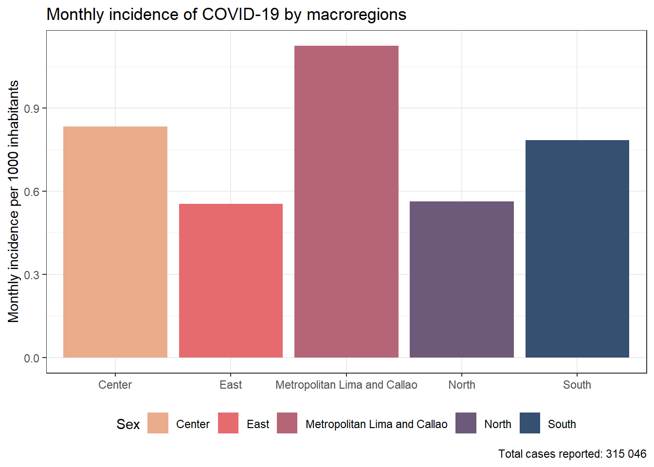
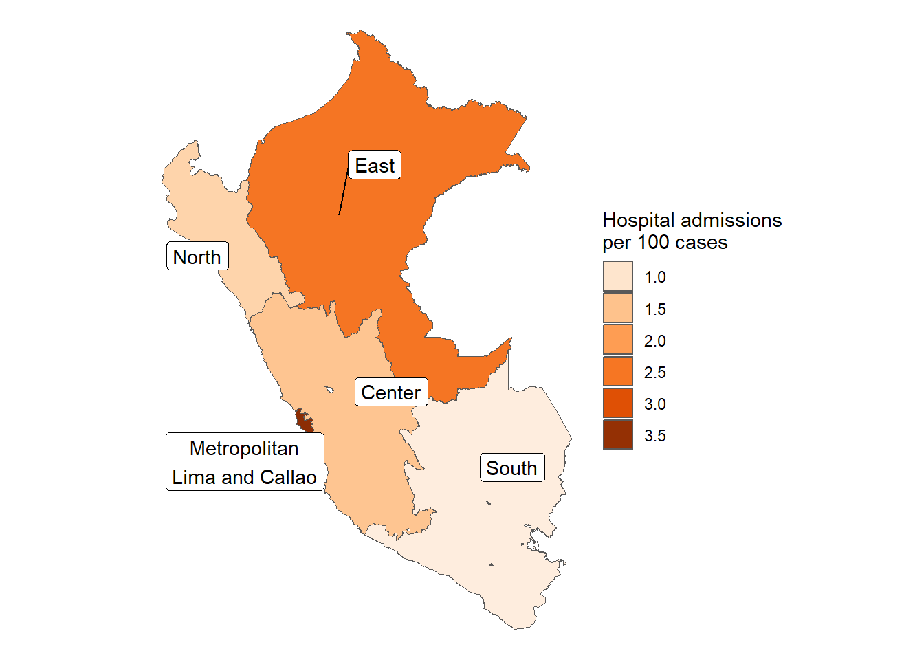
results_prevalencia$macrorregion$index %>% 
  ggplot(aes(x = macrorregion, y = rate, fill = macrorregion)) +
  geom_bar(stat = "identity") +
  theme_bw() +
  labs(title = "Monthly incidence of COVID-19 by macroregions", 
       x = NULL, 
       y = "Mean monthly COVID-19 incidence",
       fill = "Sex",
       caption = paste0("Total cases reported: ", 
                        scales::number(sum(pull(results_prevalencia$macrorregion$index_pre,
                                                count))))) +
  innovar::scale_fill_innova("blue_fall") +
  theme(
    legend.position = "bottom"
  )

Figura 13: Prevalencia COVID-19 de acuerdo a la macrorregión (07-03-2020 a 17-06-2023)

In [75]:

prev_macro_1k_sf <- peru_macro_sf %>% 
  inner_join(
    results_prevalencia$macrorregion$index
  )

Joining with `by = join_by(macrorregion)`

In [76]:

prev_macro_map <- prev_macro_1k_sf %>%
  mutate(
    macrorregion = case_match(
      macrorregion,
      "Metropolitan Lima and Callao" ~ "Met Lima & Callao",
      .default = macrorregion
    ),
    macrorregion = str_wrap(macrorregion, width = 15)
  ) %>%
  ggplot() +
  geom_sf(aes(fill = rate)) +
  ggsflabel::geom_sf_label_repel(aes(label = macrorregion),
                                 force = 100,
                                 seed = 2024) +
  guides(
    fill = guide_legend(
      str_wrap("Mean monthly COVID-19 incidence", 
               20)
    )
  ) +
  scale_fill_distiller(palette = "Oranges", # Old: YlOrBr
                       direction = 1) + 
  theme_void()

prev_macro_map

Warning in st_point_on_surface.sfc(data$geometry): st_point_on_surface may not
give correct results for longitude/latitude data

Figura 14: Prevalencia COVID-19 de acuerdo a la macrorregión (07-03-2020 a 17-06-2023)

In [77]:

In [78]:

tbl_summ_prev_macro_pre <- results_prevalencia$macrorregion$index %>% 
  mutate(
    rate = formattable::digits(rate, 3)
  ) 

tbl_summ_prev_macro <- tbl_summ_prev_macro_pre %>% 
  rename_with(
    .fn = ~ paste0("**", str_to_title(.x), "**")
  ) %>% 
  gt::gt() %>% 
  gt::cols_label(
    .fn = gt::md,
    .process_units = TRUE
  )

tbl_summ_prev_macro

Tabla 10: Prevalencia COVID-19 de acuerdo a la macrorregión (07-03-2020 a 17-06-2023)

Macrorregion	Rate
Center	0.833
East	0.555
Metropolitan Lima and Callao	1.126
North	0.564
South	0.784

In [79]:

tbl_summ_prev_macro_pre %>% 
  rename_with(
    .fn = str_to_title
  ) %>% 
  huxtable::as_hux() %>% 
  huxtable::set_bold(1, 1:2) %>% 
  huxtable::quick_xlsx(file = "02_output/tables/prevalencia_macrorregion.xlsx",
                       open = FALSE)

tbl_summ_prev_macro %>%
  gt::gtsave("02_output/tables/prevalencia_macrorregion.docx")

In [80]:

downloadthis::download_file(
  path = "02_output/tables/prevalencia_macrorregion.xlsx",
  button_label = "Descargar tabla en Excel",
  button_type = "success",
  has_icon = TRUE,
  icon = "fa fa-save"
)

In [81]:

downloadthis::download_file(
  path = "02_output/tables/prevalencia_macrorregion.docx",
  button_label = "Descargar tabla en Word",
  button_type = "primary",
  has_icon = TRUE,
  icon = "fa fa-save"
)

Distrito y sexo

In [82]:

prev_distr_sex_1k_sf <- Peru %>%
  inner_join(
    results_prevalencia$distrito_sexo$index
  ) %>%
  ungroup()

Joining with `by = join_by(ubigeo)`

In [83]:

prev_distr_sex_1k_sf %>%
  ggplot() +
  geom_sf(aes(fill = rate), 
          linewidth = 0.01,
          color = "grey75") +
  guides(
    fill = guide_legend(
      str_wrap(
        "Mean monthly COVID-19 incidence",
        20
      )
    )
  ) +
  # scale_fill_distiller(palette = "YlOrBr",
  #                      direction = 1) + 
  scale_fill_gradientn(
    colors = scales::pal_brewer("seq", "Oranges", 1)(6),
    # colors = c("#ffffcc", "#fed976", "#feb24c", "#fc4e2a", "#e31a1c", "#b10026"),
    values = scales::rescale(c(0, 25, 50, 75, 
                               100, max(prev_distr_sex_1k_sf$rate))),
    breaks = c(0, 25, 50, 75, 
               100, max(prev_distr_sex_1k_sf$rate)),
    labels = c("0", "25", "50", "75", "100", "Max"),
    limits = c(0,
               max(prev_distr_sex_1k_sf$rate))
  ) +
  facet_wrap(vars(sexo)) + 
  theme_void()

Figura 15: Prevalencia COVID-19 de acuerdo al distrito y sexo (07-03-2020 a 17-06-2023)

In [84]:

In [85]:

set.seed(2024)

tbl_summ_prev_distr_sex_pre <- results_prevalencia$distrito_sexo$index %>% 
  mutate(
    rate = formattable::digits(rate, 3)
  ) %>% 
  mutate(
    across(departamento:distrito,
           str_to_title)
  ) %>% 
  pivot_wider(
    names_from = sexo, 
    values_from = rate
  ) %>% 
  slice_sample(n = 2, by = c(departamento)) 

tbl_summ_prev_distr_sex <- tbl_summ_prev_distr_sex_pre %>% 
  rename_with(
    .fn = ~ paste0("**", str_to_title(.x), "**")
  ) %>% 
  gt::gt() %>% 
  gt::cols_label(
    .fn = gt::md,
    .process_units = TRUE
  )

tbl_summ_prev_distr_sex

Tabla 11: Prevalencia COVID-19 de acuerdo al distrito y sexo (07-03-2020 a 17-06-2023) [Tabla Recortada]

Ubigeo	Departamento	Provincia	Distrito	Female	Male
010611	Amazonas	Rodriguez De Mendoza	Totora	24.735	36.316
010503	Amazonas	Luya	Cocabamba	NA	2.481
020610	Ancash	Carhuaz	Tinco	2.571	3.203
022005	Ancash	Yungay	Quillo	0.376	0.773
030401	Apurimac	Aymaraes	Chalhuanca	4.480	2.090
030304	Apurimac	Antabamba	Juan Espinoza Medrano	4.294	4.658
040111	Arequipa	Arequipa	Mollebaya	1.943	1.523
040119	Arequipa	Arequipa	San Juan De Tarucani	6.593	5.028
050405	Ayacucho	Huanta	Luricocha	2.052	2.454
050701	Ayacucho	Parinacochas	Coracora	1.331	1.016
060203	Cajamarca	Cajabamba	Condebamba	0.788	0.934
060407	Cajamarca	Chota	Cochabamba	2.316	1.715
070102	Callao	Callao	Bellavista	4.073	4.150
070105	Callao	Callao	La Punta	6.824	6.899
080702	Cusco	Chumbivilcas	Capacmarca	1.946	3.652
080402	Cusco	Calca	Coya	2.558	1.585
090312	Huancavelica	Angaraes	Secclla	3.268	3.123
090722	Huancavelica	Tayacaja	Pichos	4.280	6.232
100101	Huanuco	Huanuco	Huanuco	0.844	0.865
100508	Huanuco	Huamalies	Punchao	1.835	1.927
110507	Ica	Pisco	San Clemente	0.816	0.959
110203	Ica	Chincha	Chavin	9.205	8.000
120203	Junin	Concepcion	Andamarca	0.979	1.201
120403	Junin	Jauja	Apata	2.323	2.686
130703	La Libertad	Pacasmayo	Jequetepeque	2.630	2.368
130906	La Libertad	Sanchez Carrion	Sanagoran	0.739	0.363
140120	Lambayeque	Chiclayo	Tuman	0.571	0.545
140203	Lambayeque	Ferrenafe	Incahuasi	0.406	0.292
150726	Lima	Huarochiri	Sangallaya	83.026	65.134
150902	Lima	Oyon	Andajes	NA	23.810
160104	Loreto	Maynas	Indiana	1.264	1.209
160107	Loreto	Maynas	Napo	3.407	3.594
170104	Madre De Dios	Tambopata	Laberinto	2.944	3.035
170301	Madre De Dios	Tahuamanu	Inapari	8.508	5.758
180211	Moquegua	General Sanchez Cerro	Yunga	13.158	12.442
180103	Moquegua	Mariscal Nieto	Cuchumbaya	32.520	14.813
190304	Pasco	Oxapampa	Palcazu	1.247	1.863
190102	Pasco	Pasco	Huachon	1.705	1.992
200704	Piura	Talara	Lobitos	12.709	6.821
200604	Piura	Sullana	Lancones	1.437	1.542
210606	Puno	Huancane	Rosaspata	NA	2.012
211207	Puno	Sandia	San Juan Del Oro	NA	2.206
220801	San Martin	Rioja	Rioja	1.942	1.700
220103	San Martin	Moyobamba	Habana	3.920	2.976
230101	Tacna	Tacna	Tacna	2.896	2.915
230106	Tacna	Tacna	Pachia	5.183	11.628
240104	Tumbes	Tumbes	Pampas De Hospital	3.231	3.748
240203	Tumbes	Contralmirante Villar	Canoas De Punta Sal	1.191	1.020
250305	Ucayali	Padre Abad	Alexander Von Humboldt	0.899	0.858
250303	Ucayali	Padre Abad	Curimana	2.193	1.950

In [86]:

tbl_summ_prev_distr_sex_pre <- results_prevalencia$distrito_sexo$index %>% 
  mutate(
    rate = formattable::digits(rate, 3)
  ) %>% 
  mutate(
    across(departamento:distrito,
           str_to_title)
  ) %>% 
  pivot_wider(
    names_from = sexo, 
    values_from = rate
  )

tbl_summ_prev_distr_sex <- tbl_summ_prev_distr_sex_pre %>% 
  rename_with(
    .fn = ~ paste0("**", str_to_title(.x), "**")
  ) %>% 
  gt::gt() %>% 
  gt::cols_label(
    .fn = gt::md,
    .process_units = TRUE
  )


tbl_summ_prev_distr_sex_pre %>% 
  rename_with(
    .fn = str_to_title
  ) %>% 
  huxtable::as_hux() %>% 
  huxtable::set_bold(1, 1:6) %>% 
  huxtable::quick_xlsx(file = "02_output/tables/prevalencia_distrito_sexo.xlsx",
                       open = FALSE)

tbl_summ_prev_distr_sex %>%
  gt::gtsave("02_output/tables/prevalencia_distrito_sexo.docx")

In [87]:

downloadthis::download_file(
  path = "02_output/tables/prevalencia_distrito_sexo.xlsx",
  button_label = "Descargar tabla en Excel",
  button_type = "success",
  has_icon = TRUE,
  icon = "fa fa-save"
)

In [88]:

downloadthis::download_file(
  path = "02_output/tables/prevalencia_distrito_sexo.docx",
  button_label = "Descargar tabla en Word",
  button_type = "primary",
  has_icon = TRUE,
  icon = "fa fa-save"
)

Distrito y edad

In [89]:

prev_distr_edad_mother <- peru_mother %>% 
  select(dep:ubigeo) %>% 
  collect() %>% 
  crossing(
    grupo_edad = levels(results_prevalencia$distrito_grupo_edad$index$grupo_edad)
  ) %>% 
  mutate(
    grupo_edad = fct_relevel(grupo_edad,
                             "Under 1 year",
                             "1 - 5 years",
                             "6 - 11 years")
  )

prev_distr_edad_100k <- prev_distr_edad_mother %>% 
  left_join(results_prevalencia$distrito_grupo_edad$index)

Joining with `by = join_by(ubigeo, grupo_edad)`

prev_distr_edad_1k_sf <- Peru %>%
  inner_join(
    prev_distr_edad_100k
  ) %>%
  ungroup()

Joining with `by = join_by(ubigeo, dep, prov, distr)`

In [90]:

prev_distr_edad_1k_sf %>%
  ggplot() +
  geom_sf(aes(fill = rate), 
          size = 0.01,
          color = "grey70") +
  guides(
    fill = guide_legend(
      str_wrap("Mean monthly COVID-19 incidence",
               20)
    )
  ) +
  # scale_fill_distiller(palette = "YlOrBr",
  #                      direction = 1) +
  # scale_fill_gradient(
  #   low = "#FEEDDE",
  #   high = "#A63603",
  #   na.value = "white"
  # ) +
  scale_fill_gradientn(
    colors = scales::pal_brewer("seq", "Oranges", 1)(6),
    # colors = c("#ffffcc", "#fed976", "#feb24c", "#fc4e2a", "#e31a1c", "#b10026"),
    values = scales::rescale(c(0, 25, 50, 75,
                               100, max(prev_distr_edad_1k_sf$rate, na.rm = TRUE))),
    breaks = c(0, 25, 50, 75,
               100, max(prev_distr_edad_1k_sf$rate, na.rm = TRUE)),
    labels = c("0", "25", "50", "75", "100", "Max"),
    limits = c(0,
               max(prev_distr_edad_1k_sf$rate, na.rm = TRUE)),
    na.value = "grey70"
  ) +
  facet_wrap(vars(grupo_edad), nrow = 1) + 
  theme_void()

Figura 16: Prevalencia COVID-19 de acuerdo al distrito y edad (07-03-2020 a 17-06-2023)

In [91]:

In [92]:

set.seed(2024)

tbl_summ_prev_distr_edad_pre <- results_prevalencia$distrito_grupo_edad$index %>% 
  mutate(
    rate = formattable::digits(rate, 3)
  ) %>% 
  mutate(
    across(departamento:distrito,
           str_to_title)
  ) %>% 
  pivot_wider(
    names_from = grupo_edad, 
    values_from = rate
  ) %>% 
  slice_sample(n = 2, by = c(departamento)) 

tbl_summ_prev_distr_edad <- tbl_summ_prev_distr_edad_pre %>% 
  rename_with(
    .fn = ~ paste0("**", str_to_title(.x), "**")
  ) %>% 
  gt::gt() %>% 
  gt::cols_label(
    .fn = gt::md,
    .process_units = TRUE
  )

tbl_summ_prev_distr_edad

Tabla 12: Prevalencia COVID-19 de acuerdo al distrito y grupo de edad (07-03-2020 a 17-06-2023) [Tabla Recortada]

Ubigeo	Departamento	Provincia	Distrito	Under 1 Year	1 - 5 Years	6 - 11 Years	12 - 17 Years
010611	Amazonas	Rodriguez De Mendoza	Totora	NA	NA	NA	34.691
010503	Amazonas	Luya	Cocabamba	NA	NA	NA	3.846
020610	Ancash	Carhuaz	Tinco	NA	5.764	3.030	3.580
022005	Ancash	Yungay	Quillo	NA	0.715	NA	0.787
030401	Apurimac	Aymaraes	Chalhuanca	11.905	3.059	2.180	7.216
030304	Apurimac	Antabamba	Juan Espinoza Medrano	NA	4.673	NA	11.825
040111	Arequipa	Arequipa	Mollebaya	16.949	2.970	1.328	4.481
040119	Arequipa	Arequipa	San Juan De Tarucani	NA	NA	9.157	12.381
050405	Ayacucho	Huanta	Luricocha	8.130	3.266	2.010	3.484
050701	Ayacucho	Parinacochas	Coracora	NA	1.146	1.192	2.067
060203	Cajamarca	Cajabamba	Condebamba	4.691	0.702	1.475	1.157
060407	Cajamarca	Chota	Cochabamba	11.236	1.946	1.826	2.772
070102	Callao	Callao	Bellavista	4.602	2.672	4.106	6.111
070105	Callao	Callao	La Punta	19.608	NA	13.525	14.205
080702	Cusco	Chumbivilcas	Capacmarca	NA	NA	5.144	2.822
080402	Cusco	Calca	Coya	NA	3.058	NA	3.012
090312	Huancavelica	Angaraes	Secclla	NA	5.597	5.682	2.045
090722	Huancavelica	Tayacaja	Pichos	NA	4.348	29.046	6.703
100101	Huanuco	Huanuco	Huanuco	1.534	0.637	0.731	1.402
100508	Huanuco	Huamalies	Punchao	15.385	6.920	NA	3.058
110507	Ica	Pisco	San Clemente	2.003	0.808	1.129	1.400
110203	Ica	Chincha	Chavin	NA	18.109	14.454	11.111
120203	Junin	Concepcion	Andamarca	8.696	NA	NA	2.218
120403	Junin	Jauja	Apata	NA	NA	2.646	5.139
130703	La Libertad	Pacasmayo	Jequetepeque	15.179	2.928	3.027	3.915
130906	La Libertad	Sanchez Carrion	Sanagoran	NA	0.532	0.602	0.641
140120	Lambayeque	Chiclayo	Tuman	2.053	0.695	0.667	0.787
140203	Lambayeque	Ferrenafe	Incahuasi	NA	NA	0.590	0.524
150726	Lima	Huarochiri	Sangallaya	125.000	57.439	105.392	130.142
150902	Lima	Oyon	Andajes	NA	NA	NA	31.250
160104	Loreto	Maynas	Indiana	3.650	1.760	1.365	1.589
160107	Loreto	Maynas	Napo	9.907	5.460	3.771	3.805
170104	Madre De Dios	Tambopata	Laberinto	16.000	4.573	3.396	4.286
170301	Madre De Dios	Tahuamanu	Inapari	20.000	6.760	9.331	13.123
180211	Moquegua	General Sanchez Cerro	Yunga	NA	17.279	11.494	23.325
180103	Moquegua	Mariscal Nieto	Cuchumbaya	NA	NA	50.000	51.656
190304	Pasco	Oxapampa	Palcazu	5.872	1.312	1.726	2.797
190102	Pasco	Pasco	Huachon	NA	4.237	3.008	2.137
200704	Piura	Talara	Lobitos	NA	NA	8.264	18.895
200604	Piura	Sullana	Lancones	4.484	1.561	2.362	2.274
210606	Puno	Huancane	Rosaspata	NA	NA	NA	3.145
211207	Puno	Sandia	San Juan Del Oro	16.949	NA	NA	4.180
220801	San Martin	Rioja	Rioja	5.768	1.860	1.369	2.868
220103	San Martin	Moyobamba	Habana	NA	4.831	5.943	6.418
230101	Tacna	Tacna	Tacna	4.890	1.680	3.095	4.215
230106	Tacna	Tacna	Pachia	25.000	9.059	10.000	5.128
240104	Tumbes	Tumbes	Pampas De Hospital	8.352	3.956	4.532	4.919
240203	Tumbes	Contralmirante Villar	Canoas De Punta Sal	NA	1.439	1.761	1.992
250305	Ucayali	Padre Abad	Alexander Von Humboldt	NA	NA	NA	1.445
250303	Ucayali	Padre Abad	Curimana	14.620	3.092	1.793	2.774

In [93]:

tbl_summ_prev_distr_edad_pre <- results_prevalencia$distrito_grupo_edad$index %>% 
  mutate(
    rate = formattable::digits(rate, 3)
  ) %>% 
  mutate(
    across(departamento:distrito,
           str_to_title)
  ) %>% 
  pivot_wider(
    names_from = grupo_edad, 
    values_from = rate
  ) 

tbl_summ_prev_distr_edad <- tbl_summ_prev_distr_edad_pre %>% 
  rename_with(
    .fn = ~ paste0("**", str_to_title(.x), "**")
  ) %>% 
  gt::gt() %>% 
  gt::cols_label(
    .fn = gt::md,
    .process_units = TRUE
  )


tbl_summ_prev_distr_edad_pre %>% 
  rename_with(
    .fn = str_to_title
  ) %>% 
  huxtable::as_hux() %>% 
  huxtable::set_bold(1, 1:6) %>% 
  huxtable::quick_xlsx(file = "02_output/tables/prevalencia_distrito_edad.xlsx",
                       open = FALSE)

tbl_summ_prev_distr_edad %>%
  gt::gtsave("02_output/tables/prevalencia_distrito_edad.docx")

In [94]:

downloadthis::download_file(
  path = "02_output/tables/prevalencia_distrito_edad.xlsx",
  button_label = "Descargar tabla en Excel",
  button_type = "success",
  has_icon = TRUE,
  icon = "fa fa-save"
)

In [95]:

downloadthis::download_file(
  path = "02_output/tables/prevalencia_distrito_edad.docx",
  button_label = "Descargar tabla en Word",
  button_type = "primary",
  has_icon = TRUE,
  icon = "fa fa-save"
)

Distrital y pobreza

In [96]:

library(biscale)

In [97]:

prev_distr_pobr_1k_sf <- Peru %>%
  inner_join(
    results_prevalencia$distrito_cuartil_pobreza$index
  ) %>%
  ungroup()

Joining with `by = join_by(ubigeo)`

prev_distr_pobr_biscale <- bi_class(prev_distr_pobr_1k_sf,
  x = rate,
  y = cuartil_pobreza,
  style = "quantile", dim = 4
)

In [98]:

custom_pal <- c(
  "1-1" = "#dae7f3", # Azul muy claro - Bajo en COVID, bajo en pobreza
  "2-1" = "#b6cee1", # Azul medio claro - Bajo en COVID, moderado en pobreza
  "3-1" = "#92b5cf", # Azul medio - Bajo en COVID, alto en pobreza
  "4-1" = "#6e9cbd", # Azul oscuro - Bajo en COVID, muy alto en pobreza
  
  
  "1-2" = "#d8f2bc", # Verde muy claro - Alto en COVID, bajo en pobreza
  "2-2" = "#a9d985", # Verde medio claro - Alto en COVID, moderado en pobreza
  "3-2" = "#7bc04e", # Verde medio - Alto en COVID, alto en pobreza
  "4-2" = "#4ca717", # Verde oscuro - Alto en COVID, muy alto en pobreza
  
  
  "1-3" = "#f8d4a0", # Naranja muy claro - Bajo en pobreza, bajo en COVID
  "2-3" = "#f6b86c", # Naranja medio claro - Moderado en pobreza, bajo en COVID
  "3-3" = "#f59b38", # Naranja medio - Alto en pobreza, bajo en COVID
  "4-3" = "#f37e04", # Naranja oscuro - Muy alto en pobreza, bajo en COVID
  

  
  "1-4" = "#f8bfcb", # Rosa muy claro - Muy alto en COVID, bajo en pobreza
  "2-4" = "#f196a0", # Rosa medio claro - Muy alto en COVID, moderado en pobreza
  "3-4" = "#ea6d75", # Rosa medio - Muy alto en COVID, alto en pobreza
  "4-4" = "#e3444a"  # Rosa oscuro - Muy alto en COVID, muy alto en pobreza
)

legend <- bi_legend(
  pal = custom_pal,
  dim = 4,
  xlab = "Incidence",
  ylab = "Poverty Quartiles",
  size = 5
)

ggmap <- prev_distr_pobr_biscale %>%
  ggplot() +
  geom_sf(aes(fill = bi_class), 
          linewidth = 0.01,
          show.legend = FALSE) +
  bi_scale_fill(pal = custom_pal, dim = 4) +
  # bi_scale_color(pal = "GrPink", dim = 3) +
  bi_theme()

library(cowplot)


Adjuntando el paquete: 'cowplot'

The following object is masked from 'package:lubridate':

    stamp

finalPlot <- ggdraw(ggmap) +
  # draw_plot(ggmap, 0, 0, 1.5, 1.5) +
  draw_plot(legend, 0.1, 0.25, 0.27, 0.27)
finalPlot

Figura 17: Prevalencia COVID-19 de acuerdo al distrito y cuartil de pobreza(07-03-2020 a 17-06-2023)

In [99]:

positivos_quartiles <- results_prevalencia$distrito_cuartil_pobreza$index %>% 
  select(prevalencia_promedio = rate, departamento, cuartil_pobreza) %>% 
  gtsummary::tbl_summary(
    by = cuartil_pobreza
  ) %>% 
  gtsummary::add_overall(last = TRUE) %>% 
  gtsummary::modify_header(label = "**Variables**") %>%
  gtsummary::bold_labels()

25 missing rows in the "cuartil_pobreza" column have been removed.

In [100]:

positivos_quartiles

Tabla 13: Cuartiles de pobreza y casos positivos menores de 18 años (07-03-2020 a 17-06-2023)

Variables	1 N = 418¹	2 N = 646¹	3 N = 531¹	4 N = 101¹	Overall N = 1,696¹
prevalencia_promedio	1.7 (1.0, 3.7)	1.9 (1.0, 4.0)	1.3 (0.8, 2.7)	0.8 (0.5, 1.7)	1.6 (0.9, 3.3)
departamento
AMAZONAS	2 (0.5%)	37 (5.7%)	33 (6.2%)	2 (2.0%)	74 (4.4%)
ANCASH	15 (3.6%)	68 (11%)	55 (10%)	10 (9.9%)	148 (8.7%)
APURIMAC	2 (0.5%)	25 (3.9%)	40 (7.5%)	0 (0%)	67 (4.0%)
AREQUIPA	59 (14%)	32 (5.0%)	8 (1.5%)	0 (0%)	99 (5.8%)
AYACUCHO	5 (1.2%)	35 (5.4%)	49 (9.2%)	10 (9.9%)	99 (5.8%)
CAJAMARCA	1 (0.2%)	11 (1.7%)	51 (9.6%)	53 (52%)	116 (6.8%)
CALLAO	4 (1.0%)	2 (0.3%)	0 (0%)	0 (0%)	6 (0.4%)
CUSCO	13 (3.1%)	54 (8.4%)	38 (7.2%)	1 (1.0%)	106 (6.3%)
HUANCAVELICA	5 (1.2%)	41 (6.3%)	37 (7.0%)	3 (3.0%)	86 (5.1%)
HUANUCO	8 (1.9%)	32 (5.0%)	33 (6.2%)	1 (1.0%)	74 (4.4%)
ICA	41 (9.8%)	1 (0.2%)	0 (0%)	0 (0%)	42 (2.5%)
JUNIN	29 (6.9%)	78 (12%)	11 (2.1%)	0 (0%)	118 (7.0%)
LA LIBERTAD	11 (2.6%)	25 (3.9%)	29 (5.5%)	10 (9.9%)	75 (4.4%)
LAMBAYEQUE	23 (5.5%)	12 (1.9%)	2 (0.4%)	1 (1.0%)	38 (2.2%)
LIMA	103 (25%)	45 (7.0%)	1 (0.2%)	0 (0%)	149 (8.8%)
LORETO	2 (0.5%)	12 (1.9%)	38 (7.2%)	1 (1.0%)	53 (3.1%)
MADRE DE DIOS	11 (2.6%)	0 (0%)	0 (0%)	0 (0%)	11 (0.6%)
MOQUEGUA	11 (2.6%)	8 (1.2%)	0 (0%)	0 (0%)	19 (1.1%)
PASCO	2 (0.5%)	12 (1.9%)	14 (2.6%)	1 (1.0%)	29 (1.7%)
PIURA	13 (3.1%)	27 (4.2%)	20 (3.8%)	4 (4.0%)	64 (3.8%)
PUNO	2 (0.5%)	29 (4.5%)	64 (12%)	4 (4.0%)	99 (5.8%)
SAN MARTIN	21 (5.0%)	48 (7.4%)	7 (1.3%)	0 (0%)	76 (4.5%)
TACNA	12 (2.9%)	7 (1.1%)	0 (0%)	0 (0%)	19 (1.1%)
TUMBES	13 (3.1%)	0 (0%)	0 (0%)	0 (0%)	13 (0.8%)
UCAYALI	10 (2.4%)	5 (0.8%)	1 (0.2%)	0 (0%)	16 (0.9%)
¹ Median (Q1, Q3); n (%)

In [101]:

positivos_quartiles %>% 
  gtsummary::as_hux_xlsx("02_output/tables/prevalencia_distritos_pobreza_descriptivos_by_dep.xlsx")

positivos_quartiles %>%
  gtsummary::as_flex_table() %>%
  flextable::save_as_docx(path = "02_output/tables/prevalencia_distritos_pobreza_descriptivos_by_dep.docx")

In [102]:

downloadthis::download_file(
  path = "02_output/tables/prevalencia_distritos_pobreza_descriptivos_by_dep.xlsx",
  button_label = "Descargar tabla en Excel",
  button_type = "success",
  has_icon = TRUE,
  icon = "fa fa-save"
)

In [103]:

downloadthis::download_file(
  path = "02_output/tables/prevalencia_distritos_pobreza_descriptivos_by_dep.docx",
  button_label = "Descargar tabla en Word",
  button_type = "primary",
  has_icon = TRUE,
  icon = "fa fa-save"
)

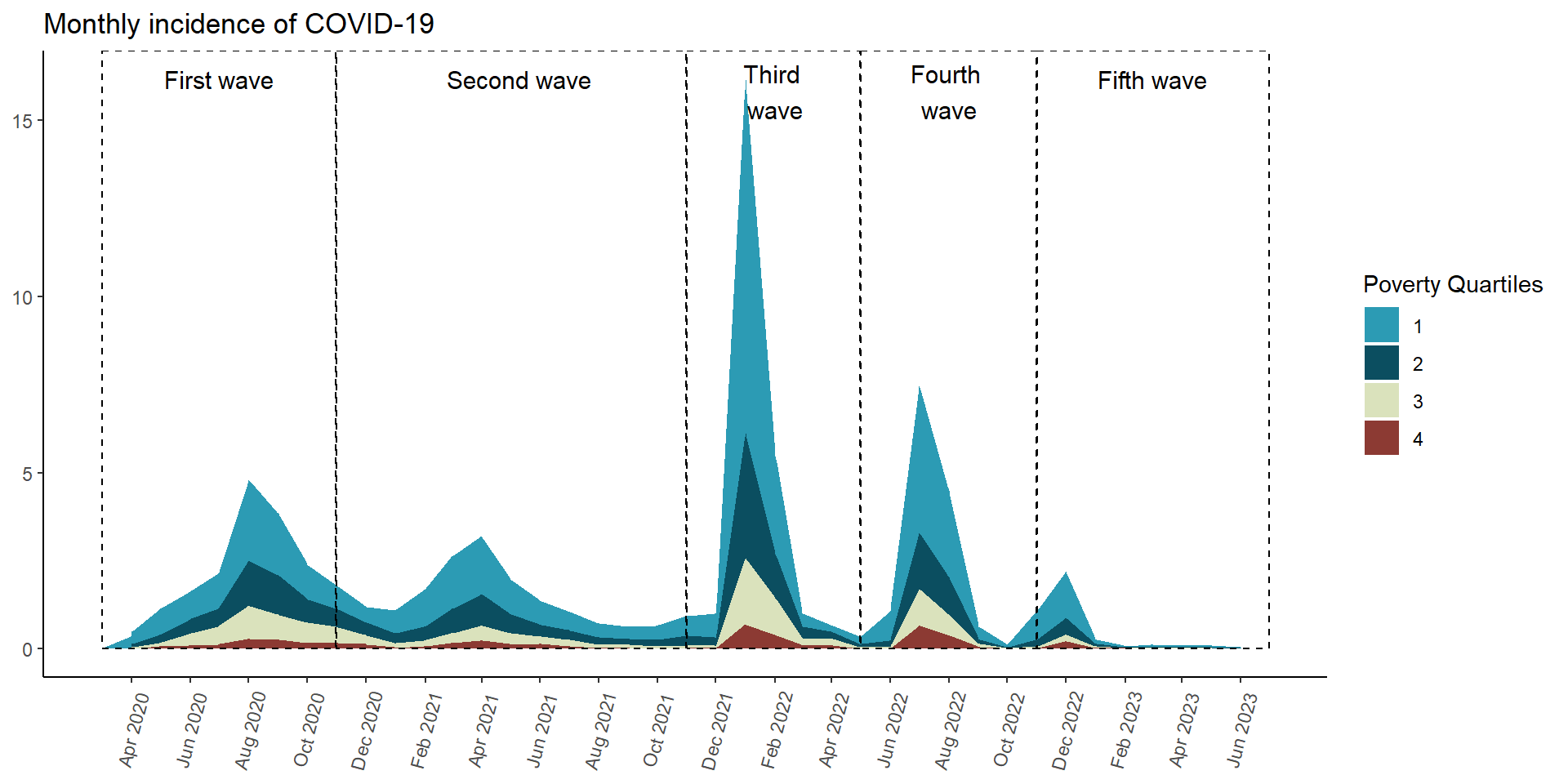
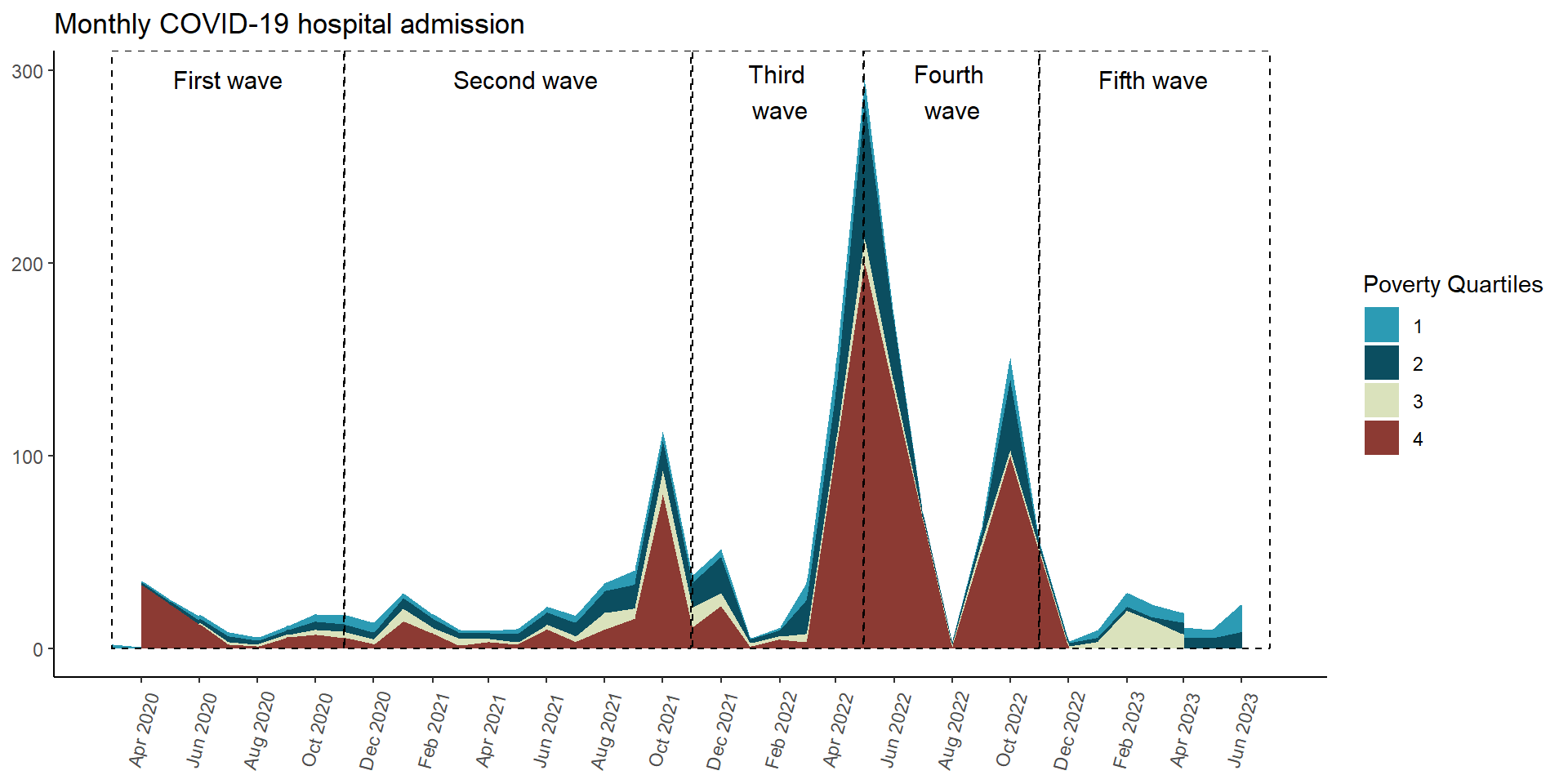
In [104]:

prev_pobr_area_plot <- 
  results_per_month_prevalencia$cuartil_pobreza$index %>% 
  drop_na() %>% 
  mutate(
    time = make_date(anio, mes, "1")
  ) %>% 
  ggplot(
    aes(x = time,
        y = rate,
        fill = cuartil_pobreza)
  ) +
  geom_area(position = 'stack') +
  # innovar::scale_fill_innova("jama") +
  scale_fill_manual(
    values = c("#2C9BB4", "#0B4E60", "#DAE2BC", "#8C3A33")
  ) +
  scale_x_date(
    limits = c(ymd("2020-03-01"), ymd("2023-07-01")),
    breaks = seq(from = ceiling_date(ymd("2020-03-01"), "month"),
                 to = floor_date(ymd("2023-07-01"), "month"),
                 by = "2 months"), 
    # date_breaks = "2 month",
    date_labels = "%b %Y"
  ) +
  labs(
    y = NULL,
    x = NULL,
    title = "Monthly incidence of COVID-19",
    fill = "Poverty Quartiles"
  ) + 
  annotate(
    geom = "rect",
    xmin = as.Date("2020-03-01"), 
    xmax = as.Date("2020-10-31"), 
    ymin = 0, # El rectángulo se extiende hasta la parte inferior del gráfico
    ymax = Inf, # El rectángulo se extiende hasta la parte superior del gráfico
    color = "black", # Color de la línea
    fill = NA, # Sin relleno
    linetype = "dashed", # Tipo de línea discontinua
    linewidth = 0.5 # Grosor de la línea
  ) + 
  annotate(
    geom = "text", 
    x = as.Date("2020-07-01"), # Punto medio aproximado de la Ola 2
    y = Inf, # Posición vertical del texto
    label = "First wave", 
    color = "black",
    size = 4, # Tamaño del texto
    vjust = 2 # Ajuste vertical para colocar el texto encima del rectángulo
  ) +
  annotate(
    geom = "rect",
    xmin = as.Date("2020-11-01"), 
    xmax = as.Date("2021-10-31"), 
    ymin = 0, # El rectángulo se extiende hasta la parte inferior del gráfico
    ymax = Inf, # El rectángulo se extiende hasta la parte superior del gráfico
    color = "black", # Color de la línea
    fill = NA, # Sin relleno
    linetype = "dashed", # Tipo de línea discontinua
    linewidth = 0.5 # Grosor de la línea
  ) + 
  annotate(
    geom = "text", 
    x = as.Date("2021-05-10"), # Punto medio aproximado de la Ola 2
    y = Inf, # Posición vertical del texto
    label = "Second wave", 
    color = "black",
    size = 4, # Tamaño del texto
    vjust = 2 # Ajuste vertical para colocar el texto encima del rectángulo
  ) + 
  annotate(
    geom = "rect",
    xmin = as.Date("2021-11-01"), 
    xmax = as.Date("2022-04-30"), 
    ymin = 0, # El rectángulo se extiende hasta la parte inferior del gráfico
    ymax = Inf, # El rectángulo se extiende hasta la parte superior del gráfico
    color = "black", # Color de la línea
    fill = NA, # Sin relleno
    linetype = "dashed", # Tipo de línea discontinua
    linewidth = 0.5 # Grosor de la línea
  ) + 
  annotate(
    geom = "text", 
    x = as.Date("2022-02-01"), # Punto medio aproximado de la Ola 2
    y = Inf, # Posición vertical del texto
    label = "Third \nwave", 
    color = "black",
    size = 4, # Tamaño del texto
    vjust = 1.25 # Ajuste vertical para colocar el texto encima del rectángulo
  ) + 
  annotate(
    geom = "rect",
    xmin = as.Date("2022-05-01"), 
    xmax = as.Date("2022-10-31"), 
    ymin = 0, # El rectángulo se extiende hasta la parte inferior del gráfico
    ymax = Inf, # El rectángulo se extiende hasta la parte superior del gráfico
    color = "black", # Color de la línea
    fill = NA, # Sin relleno
    linetype = "dashed", # Tipo de línea discontinua
    linewidth = 0.5 # Grosor de la línea
  ) + 
  annotate(
    geom = "text", 
    x = as.Date("2022-08-01"), # Punto medio aproximado de la Ola 2
    y = Inf, # Posición vertical del texto
    label = "Fourth \nwave", 
    color = "black",
    size = 4, # Tamaño del texto
    vjust = 1.25 # Ajuste vertical para colocar el texto encima del rectángulo
  ) +
  annotate(
    geom = "rect",
    xmin = as.Date("2022-11-01"), 
    xmax = as.Date("2023-07-01"), 
    ymin = 0, # El rectángulo se extiende hasta la parte inferior del gráfico
    ymax = Inf, # El rectángulo se extiende hasta la parte superior del gráfico
    color = "black", # Color de la línea
    fill = NA, # Sin relleno
    linetype = "dashed", # Tipo de línea discontinua
    linewidth = 0.5 # Grosor de la línea
  ) + 
  annotate(
    geom = "text", 
    x = as.Date("2023-03-01"),
    y = Inf, # Posición vertical del texto
    label = "Fifth wave", 
    color = "black",
    size = 4, # Tamaño del texto
    vjust = 2 # Ajuste vertical para colocar el texto encima del rectángulo
  ) +
  theme_classic() +
  theme(
    axis.text.x = element_text(
      angle = 75,
      vjust = 0.5
    ),
    axis.ticks.x = element_line()
  ) 

prev_pobr_area_plot

Figura 18: Prevalencia COVID-19 de acuerdo al cuartil de pobreza(07-03-2020 a 17-06-2023)

Distrito Lima

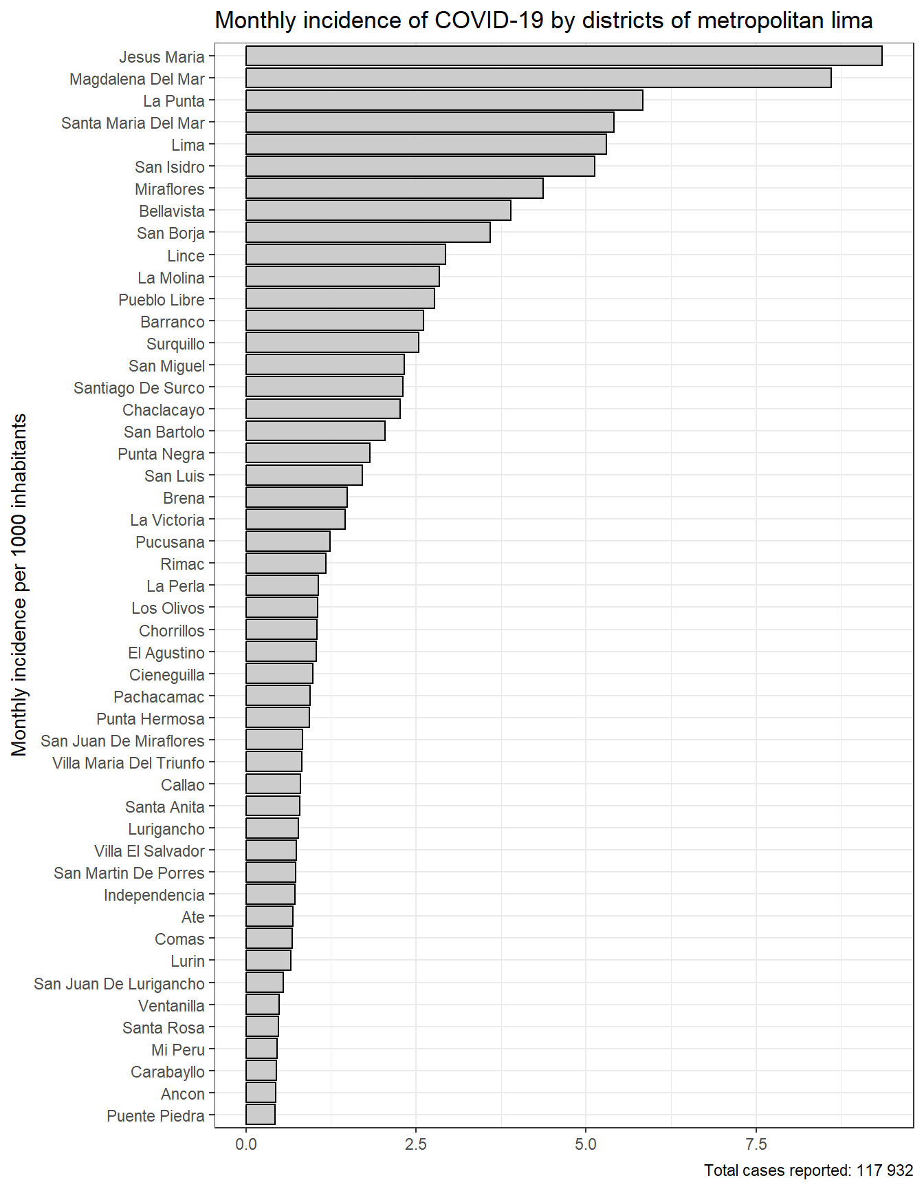
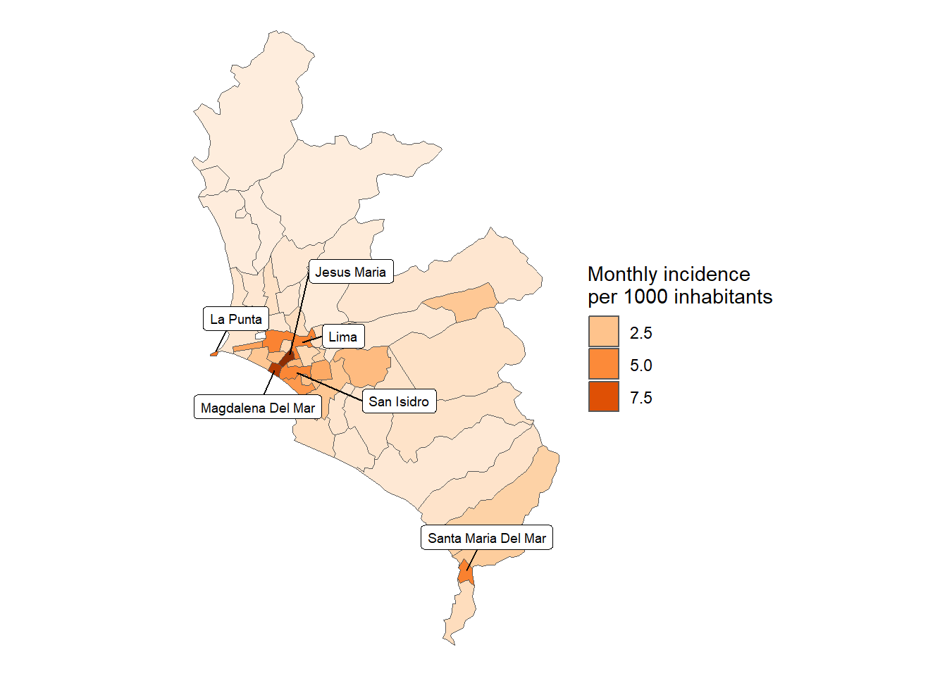
In [105]:

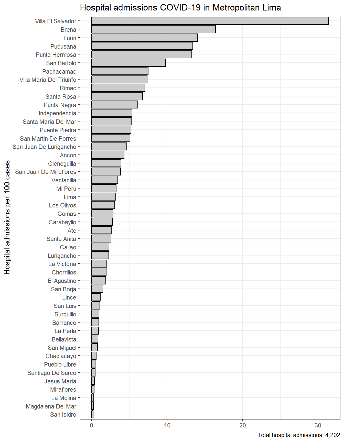
total_cases_distr_lim_callao <- results_prevalencia$distrito$index_pre %>% 
  filter(provincia %in% c("LIMA", "CALLAO")) %>% 
  pull(count) %>% 
  sum()

results_prevalencia$distrito$index %>% 
  filter(provincia %in% c("LIMA", "CALLAO")) %>% 
  mutate(
    distrito = str_to_title(distrito), 
    distrito = fct_reorder(distrito, rate)
  ) %>% 
  ggplot(aes(y = distrito, x = rate)) +
  geom_bar(stat = "identity",
           color = "black",
           fill = "grey80") +
  theme_bw() +
  labs(title = "Monthly incidence of COVID-19 by districts of metropolitan lima", 
       x = NULL, 
       y = "Mean monthly COVID-19 incidence",
       caption = paste0("Total cases reported: ", 
                        scales::number(total_cases_distr_lim_callao))) +
  innovar::scale_fill_innova("blue_fall") +
  theme(
    legend.position = "bottom"
  )

Figura 19: Prevalencia COVID-19 de acuerdo a los distritos de lima metropolitana (07-03-2020 a 17-06-2023)

In [106]:

prev_lima_distr_1k_sf <- Peru %>% 
  inner_join(
    results_prevalencia$distrito$index %>% 
      filter(provincia %in% c("LIMA", "CALLAO"))
  )

Joining with `by = join_by(ubigeo)`

In [107]:

prev_lima_distr_1k_sf %>%
  mutate(
    label = case_when(
      rate > 5 ~ str_to_title(distrito)
    )
  ) %>% 
  ggplot() +
  geom_sf(aes(fill = rate)) +
  guides(
    fill = guide_legend(
      str_wrap("Mean monthly COVID-19 incidence", 
               20)
    )
  ) +
  ggsflabel::geom_sf_label_repel(aes(label = label),
                                 force = 10,
                                 size = 2.45,
                                 box.padding = 0.75,
                                 seed = 2024) +
  scale_fill_distiller(palette = "Oranges", # Old: YlOrBr
                       direction = 1) + 
  theme_void()

Warning in st_point_on_surface.sfc(data$geometry): st_point_on_surface may not
give correct results for longitude/latitude data

Warning: Removed 43 rows containing missing values or values outside the scale range
(`geom_label_repel()`).

Figura 20: Prevalencia COVID-19 de acuerdo a los distritos de lima metropolitana (07-03-2020 a 17-06-2023)

In [108]:

In [109]:

tbl_summ_prev_lima_distr_pre <- results_prevalencia$distrito$index %>% 
      filter(provincia %in% c("LIMA", "CALLAO")) %>% 
  mutate(
    across(
      departamento:distrito,
      str_to_title
    ),
    rate = formattable::digits(rate, 3)
  ) %>% 
  select(-departamento)

tbl_summ_prev_lima_distr <- tbl_summ_prev_lima_distr_pre %>% 
  rename_with(
    .fn = ~ paste0("**", str_to_title(.x), "**")
  ) %>% 
  gt::gt() %>% 
  gt::cols_label(
    .fn = gt::md,
    .process_units = TRUE
  )

tbl_summ_prev_lima_distr

Tabla 14: Prevalencia COVID-19 de acuerdo a los distritos de lima metropolitana (07-03-2020 a 17-06-2023)

Ubigeo	Provincia	Distrito	Rate
070101	Callao	Callao	0.801
070102	Callao	Bellavista	3.890
070104	Callao	La Perla	1.065
070105	Callao	La Punta	5.831
070106	Callao	Ventanilla	0.483
070107	Callao	Mi Peru	0.459
150101	Lima	Lima	5.294
150102	Lima	Ancon	0.439
150103	Lima	Ate	0.692
150104	Lima	Barranco	2.611
150105	Lima	Brena	1.485
150106	Lima	Carabayllo	0.445
150107	Lima	Chaclacayo	2.267
150108	Lima	Chorrillos	1.045
150109	Lima	Cieneguilla	0.987
150110	Lima	Comas	0.676
150111	Lima	El Agustino	1.038
150112	Lima	Independencia	0.723
150113	Lima	Jesus Maria	9.348
150114	Lima	La Molina	2.844
150115	Lima	La Victoria	1.459
150116	Lima	Lince	2.933
150117	Lima	Los Olivos	1.048
150118	Lima	Lurigancho	0.772
150119	Lima	Lurin	0.659
150120	Lima	Magdalena Del Mar	8.608
150121	Lima	Pueblo Libre	2.776
150122	Lima	Miraflores	4.366
150123	Lima	Pachacamac	0.943
150124	Lima	Pucusana	1.240
150125	Lima	Puente Piedra	0.425
150126	Lima	Punta Hermosa	0.929
150127	Lima	Punta Negra	1.820
150128	Lima	Rimac	1.172
150129	Lima	San Bartolo	2.044
150130	Lima	San Borja	3.594
150131	Lima	San Isidro	5.130
150132	Lima	San Juan De Lurigancho	0.550
150133	Lima	San Juan De Miraflores	0.827
150134	Lima	San Luis	1.712
150135	Lima	San Martin De Porres	0.726
150136	Lima	San Miguel	2.326
150137	Lima	Santa Anita	0.794
150138	Lima	Santa Maria Del Mar	5.405
150139	Lima	Santa Rosa	0.478
150140	Lima	Santiago De Surco	2.310
150141	Lima	Surquillo	2.539
150142	Lima	Villa El Salvador	0.735
150143	Lima	Villa Maria Del Triunfo	0.818

In [110]:

tbl_summ_prev_lima_distr_pre %>% 
  rename_with(
    .fn = str_to_title
  ) %>% 
  huxtable::as_hux() %>% 
  huxtable::set_bold(1, 1:4) %>% 
  huxtable::quick_xlsx(file = "02_output/tables/prevalencia_lima_distrito.xlsx",
                       open = FALSE)

tbl_summ_prev_lima_distr %>%
  gt::gtsave("02_output/tables/prevalencia_lima_distrito.docx")

In [111]:

downloadthis::download_file(
  path = "02_output/tables/prevalencia_lima_distrito.xlsx",
  button_label = "Descargar tabla en Excel",
  button_type = "success",
  has_icon = TRUE,
  icon = "fa fa-save"
)

In [112]:

downloadthis::download_file(
  path = "02_output/tables/prevalencia_lima_distrito.docx",
  button_label = "Descargar tabla en Word",
  button_type = "primary",
  has_icon = TRUE,
  icon = "fa fa-save"
)

Fallecidos - Mortalidad

In [113]:

fallecidos_total <- fallecidos_total %>% 
  filter(
    edad_declarada < 18,
    fecha_fallecimiento <= max_positivos_0723
  ) %>% 
  mutate(
    dep.code = str_sub(ubigeo, 1, 2),
    overall = "overall"
  ) 

range_fallecidos <- fallecidos_total %>% 
  summarise(
    min = min(fecha_fallecimiento),
    max = max(fecha_fallecimiento)
  ) %>% 
  collect() %>% 
  mutate(
    min = format(min, "%d-%m-%Y"),
    max = format(max, "%d-%m-%Y"),
    fecha = paste0("(", min, " a ", max, ")")
  )

Vista general

Cálculo de mortalidad

In [114]:

levels <- list(
  c("overall"),
  c("grupo_edad"),
  c("sexo"),
  c("grupo_edad", "sexo"),
  c("ola_covid"),
  c("ola_covid", "grupo_edad"),
  c("ola_covid", "sexo"),
  c("ola_covid", "region"),
  c("ola_covid", "macrorregion"),
  c("departamento"),
  c("departamento", "sexo"),
  c("departamento", "grupo_edad"),
  c("departamento", "sexo", "grupo_edad"),
  c("departamento", "ola_covid"),
  c("distrito"),
  c("distrito", "sexo"),
  c("distrito", "grupo_edad"),
  c("distrito", "cuartil_pobreza"),
  c("grupo_edad", "cuartil_pobreza"),
  c("sexo", "cuartil_pobreza"),
  c("ola_covid", "cuartil_pobreza"),
  c("ola_covid", "cuartil_nbi"),
  c("cuartil_pobreza"),
  c("cuartil_nbi"),
  c("region"),
  c("macrorregion")
)

# Calcular la mortalidad
results_mortalidad <- index_calculator(
  data = fallecidos_total, 
  denom = poblacion %>% mutate(overall = "overall"), 
  levels = levels, 
  type = "month",
  std = 100000
)

results_per_month_mortalidad <- index_calculator(
  data = fallecidos_total, 
  denom = poblacion %>% mutate(overall = "overall"), 
  levels = levels, 
  type = "per_month",
  std = 100000
)

Cálculo de letalidad

In [115]:

# Calcular la letalidad
results_letalidad_mensual <- index_calculator(
  data = fallecidos_total, 
  denom = positivos_0723 %>% 
    mutate(cantidad = 1), 
  levels = levels, 
  type = "month",
  std = 100
)

results_per_month_letalidad <- index_calculator(
  data = fallecidos_total, 
  denom = positivos_0723 %>% 
    mutate(cantidad = 1), 
  levels = levels, 
  type = "per_month",
  std = 100
)

results_letalidad_overall <- index_calculator(
  data = fallecidos_total, 
  denom = positivos_0723 %>% 
    mutate(cantidad = 1), 
  levels = levels, 
  type = "overall",
  std = 100
)

In [116]:

fallecidos_total_df <- fallecidos_total %>% 
  select(overall, edad_declarada, grupo_edad, sexo, ola_covid, region, 
         macrorregion, cuartil_pobreza, cuartil_nbi) %>% 
  collect()

labelled::var_label(fallecidos_total_df) <- list(
  overall = "Overall",
  grupo_edad = "Age Group",
  sexo = "Sex",
  ola_covid = "COVID-19 wave",
  region = "Natural Regions",
  macrorregion = "Macroregions",
  cuartil_pobreza = "Poverty level",
  cuartil_nbi = "Unsatisfied basic needs level"
)

In [117]:

tbl_summ_fallecidos_g <- fallecidos_total_df %>% 
  select(-edad_declarada) %>% 
  gtsummary::tbl_summary(
    type = list(
      overall ~ "dichotomous"
    ),
    value = list(overall = "overall"),
    missing_text = "No data"
  ) %>% 
  gtsummary::modify_header(label = "**Variables**") %>%
  gtsummary::bold_labels()

tbl_summ_fallecidos_c2 <- results_mortalidad$overall$index %>% 
  mutate(label = "Overall") %>% 
  rename(variable = overall) %>% 
  bind_rows(
    results_mortalidad$grupo_edad$index %>% 
      mutate(variable = "grupo_edad") %>% 
      rename(label = grupo_edad),
    results_mortalidad$sexo$index %>% 
      mutate(variable = "sexo") %>% 
      rename(label = sexo),
    results_mortalidad$ola_covid$index %>% 
      mutate(variable = "ola_covid") %>% 
      rename(label = ola_covid),
    results_mortalidad$region$index %>% 
      mutate(variable = "region") %>% 
      rename(label = region),
    results_mortalidad$macrorregion$index %>% 
      mutate(variable = "macrorregion") %>% 
      rename(label = macrorregion),
    results_mortalidad$cuartil_pobreza$index %>% 
      mutate(variable = "cuartil_pobreza") %>% 
      rename(label = cuartil_pobreza),
    results_mortalidad$cuartil_nbi$index %>% 
      mutate(variable = "cuartil_nbi") %>% 
      rename(label = cuartil_nbi)
  ) %>% 
  drop_na() %>% 
  mutate(
    rate = formattable::digits(rate, 3)
  )

tbl_summ_fallecidos_c3 <- results_letalidad_mensual$overall$index %>% 
  mutate(label = "Overall") %>% 
  rename(variable = overall) %>% 
  bind_rows(
    results_letalidad_mensual$grupo_edad$index %>% 
      mutate(variable = "grupo_edad") %>% 
      rename(label = grupo_edad),
    results_letalidad_mensual$sexo$index %>% 
      mutate(variable = "sexo") %>% 
      rename(label = sexo),
    results_letalidad_mensual$ola_covid$index %>% 
      mutate(variable = "ola_covid") %>% 
      rename(label = ola_covid),
    results_letalidad_mensual$region$index %>% 
      mutate(variable = "region") %>% 
      rename(label = region),
    results_letalidad_mensual$macrorregion$index %>% 
      mutate(variable = "macrorregion") %>% 
      rename(label = macrorregion),
    results_letalidad_mensual$cuartil_pobreza$index %>% 
      mutate(variable = "cuartil_pobreza") %>% 
      rename(label = cuartil_pobreza),
    results_letalidad_mensual$cuartil_nbi$index %>% 
      mutate(variable = "cuartil_nbi") %>% 
      rename(label = cuartil_nbi)
  ) %>% 
  drop_na() %>% 
  mutate(
    rate = formattable::digits(rate, 3)
  ) %>% 
  rename(letalidad_mensual = rate)

tbl_summ_fallecidos_c4 <- results_letalidad_overall$overall$index %>% 
  mutate(label = "Overall") %>% 
  rename(variable = overall) %>% 
  bind_rows(
    results_letalidad_overall$grupo_edad$index %>% 
      mutate(variable = "grupo_edad") %>% 
      rename(label = grupo_edad),
    results_letalidad_overall$sexo$index %>% 
      mutate(variable = "sexo") %>% 
      rename(label = sexo),
    results_letalidad_overall$ola_covid$index %>% 
      mutate(variable = "ola_covid") %>% 
      rename(label = ola_covid),
    results_letalidad_overall$region$index %>% 
      mutate(variable = "region") %>% 
      rename(label = region),
    results_letalidad_overall$macrorregion$index %>% 
      mutate(variable = "macrorregion") %>% 
      rename(label = macrorregion),
    results_letalidad_overall$cuartil_pobreza$index %>% 
      mutate(variable = "cuartil_pobreza") %>% 
      rename(label = cuartil_pobreza),
    results_letalidad_overall$cuartil_nbi$index %>% 
      mutate(variable = "cuartil_nbi") %>% 
      rename(label = cuartil_nbi)
  ) %>% 
  drop_na() %>% 
  mutate(
    rate = formattable::digits(rate, 3)
  ) %>% 
  rename(letalidad_overall = rate)


tbl_summ_fallecidos_final <- tbl_summ_fallecidos_g %>%
  gtsummary::modify_table_body(
    ~ .x %>% 
      left_join(tbl_summ_fallecidos_c2) %>% 
      left_join(tbl_summ_fallecidos_c3) %>% 
      left_join(tbl_summ_fallecidos_c4) %>% 
      mutate(
        label = case_when(
          variable %in% c("cuartil_pobreza", "cuartil_nbi") &
            label == "1" ~ "1 (0-19.9%)",
          variable %in% c("cuartil_pobreza", "cuartil_nbi") & 
            label == "2" ~ "2 (20-39.9%)",
          variable %in% c("cuartil_pobreza", "cuartil_nbi") & 
            label == "3" ~ "3 (40-59.9%)",
          variable %in% c("cuartil_pobreza", "cuartil_nbi") &
            label == "4" ~ "4 (60-100%)",
          .default = label
        )
      )
  ) %>% 
  gtsummary::modify_header(
    rate ~ "**Average monthly mortality per 100K habitants**",
    letalidad_mensual ~ "**Average monthly lethality per 100 cases**",
    letalidad_overall ~ "**Lethality per 100 cases**"
  )

Joining with `by = join_by(variable, label)`
Joining with `by = join_by(variable, label)`
Joining with `by = join_by(variable, label)`

In [118]:

tbl_summ_fallecidos_final

Tabla 15: Descriptivos de fallecidos menores de 18 años (14-03-2020 a 13-06-2023)

Variables	N = 1,616¹	Average monthly mortality per 100K habitants	Average monthly lethality per 100 cases	Lethality per 100 cases
Overall	1,616 (100%)	0.412	1.310	0.513
Age Group
Under 1 year	251 (16%)	1.327	2.732	1.518
1 - 5 years	496 (31%)	0.470	2.765	1.088
6 - 11 years	393 (24%)	0.300	1.434	0.429
12 - 17 years	476 (29%)	0.375	0.793	0.295
Sex
Female	729 (45%)	0.374	1.145	0.457
Male	887 (55%)	0.450	1.460	0.571
COVID-19 wave
1 (Mar – Oct 2020)	589 (36%)	0.769	3.172	0.983
2 (Nov 2020 – Oct 2021)	588 (36%)	0.482	0.813	0.811
3 (Nov 2021 – Apr 2022)	230 (14%)	0.397	0.553	0.216
4 (May 2022 – Oct 2022)	144 (8.9%)	0.251	0.745	0.248
5 (Nov 2022 – Jun 2023)	65 (4.0%)	0.081	1.185	0.358
Natural Regions
Coast	998 (62%)	0.427	0.994	0.426
Highlands	366 (23%)	0.351	1.244	0.678
Jungle	252 (16%)	0.668	7.180	0.947
Macroregions
Center	312 (19%)	0.363	1.290	0.433
East	232 (14%)	0.644	6.675	0.950
Metropolitan Lima and Callao	491 (30%)	0.466	1.018	0.415
North	358 (22%)	0.430	2.878	0.708
South	223 (14%)	0.418	3.891	0.449
Poverty level
1 (0-19.9%)	1,022 (63%)	0.470	1.024	0.438
2 (20-39.9%)	388 (24%)	0.394	1.337	0.780
3 (40-59.9%)	174 (11%)	0.395	5.777	1.155
4 (60-100%)	32 (2.0%)	0.642	18.733	2.168
Unsatisfied basic needs level
1 (0-19.9%)	727 (45%)	0.434	0.933	0.384
2 (20-39.9%)	567 (35%)	0.404	1.598	0.700
3 (40-59.9%)	219 (14%)	0.490	4.290	1.218
4 (60-100%)	103 (6.4%)	0.529	3.670	0.927
¹ n (%)

In [119]:

tbl_summ_fallecidos_final %>% 
  gtsummary::as_hux_xlsx("02_output/tables/fallecidos_descriptivos.xlsx")

tbl_summ_fallecidos_final %>%
  gtsummary::as_flex_table() %>%
  flextable::save_as_docx(path = "02_output/tables/fallecidos_descriptivos.docx")

In [120]:

downloadthis::download_file(
  path = "02_output/tables/fallecidos_descriptivos.xlsx",
  button_label = "Descargar tabla en Excel",
  button_type = "success",
  has_icon = TRUE,
  icon = "fa fa-save"
)

In [121]:

downloadthis::download_file(
  path = "02_output/tables/fallecidos_descriptivos.docx",
  button_label = "Descargar tabla en Word",
  button_type = "primary",
  has_icon = TRUE,
  icon = "fa fa-save"
)

In [122]:

mortality_comparisons <- compare_levels_per_month(
  results_per_month = results_per_month_mortalidad,
  levels = comparing_levels
)

# Extraer las tablas `cld` como tibbles, renombrando y añadiendo una columna "level"
mortality_comparisons_cld_pre <- lapply(names(mortality_comparisons), function(level) {
  cld <- mortality_comparisons[[level]]$cld
  
  if (!is.null(cld)) {
    cld <- cld |> 
      as_tibble() |> 
      rename(group = 1) |>  # Renombra la primera columna a 'group'
      mutate(level = level) |> # Añade una columna 'level' con el nombre de la lista
      relocate(level) 
  }
  
  cld
}) |> 
  bind_rows()

mortality_comparisons_cld_pre <- 
  mortality_comparisons_cld_pre |> 
  mutate(
    across(
      where(is.numeric),
      ~ formattable::digits(.x, 3)
    )
  )

In [123]:

In [124]:

mortality_comparisons_cld <- mortality_comparisons_cld_pre |> 
  rename_with(
    .fn = ~ paste0("**", str_to_title(.x), "**")
  ) %>% 
  gt::gt() %>% 
  gt::cols_label(
    .fn = gt::md,
    .process_units = TRUE
  )

mortality_comparisons_cld

Tabla 16: Comparaciones múltiples de mortalidad(07-03-2020 a 17-06-2023)

Level	Group	Emmean	Se	Df	Lower.cl	Upper.cl	.Group
grupo_edad	6 - 11 years	0.300	0.106	110.010	0.090	0.510	a
grupo_edad	12 - 17 years	0.366	0.107	111.863	0.154	0.578	a
grupo_edad	1 - 5 years	0.458	0.108	113.597	0.243	0.673	a
grupo_edad	Under 1 year	1.314	0.109	115.492	1.097	1.530	b
sexo	Female	0.374	0.054	43.889	0.265	0.483	a
sexo	Male	0.450	0.054	43.889	0.341	0.559	b
ola_covid	5 (Nov 2022 – Jun 2023)	0.081	0.089	35.000	-0.099	0.262	a
ola_covid	4 (May 2022 – Oct 2022)	0.251	0.102	35.000	0.043	0.459	ab
ola_covid	3 (Nov 2021 – Apr 2022)	0.397	0.102	35.000	0.189	0.605	abc
ola_covid	2 (Nov 2020 – Oct 2021)	0.482	0.072	35.000	0.334	0.629	bc
ola_covid	1 (Mar – Oct 2020)	0.769	0.089	35.000	0.589	0.949	c
cuartil_pobreza	3	0.340	0.058	82.220	0.225	0.456	a
cuartil_pobreza	2	0.378	0.055	73.977	0.268	0.489	a
cuartil_pobreza	1	0.470	0.054	69.740	0.363	0.578	a
cuartil_pobreza	4	0.515	0.073	115.495	0.371	0.660	a
cuartil_nbi	2	0.404	0.057	54.319	0.289	0.519	a
cuartil_nbi	4	0.422	0.061	68.351	0.299	0.544	a
cuartil_nbi	3	0.433	0.059	61.864	0.314	0.552	a
cuartil_nbi	1	0.434	0.057	54.319	0.320	0.549	a
region	Highlands	0.337	0.069	70.603	0.200	0.474	a
region	Coast	0.427	0.067	66.848	0.293	0.562	a
region	Jungle	0.637	0.071	76.304	0.495	0.779	b
macrorregion	Center	0.355	0.064	75.310	0.227	0.483	a
macrorregion	South	0.359	0.067	85.511	0.226	0.492	a
macrorregion	North	0.404	0.065	78.327	0.275	0.534	a
macrorregion	Metropolitan Lima and Callao	0.466	0.064	73.873	0.339	0.593	ab
macrorregion	East	0.601	0.067	85.448	0.468	0.734	b

In [125]:

mortality_comparisons_cld_pre %>% 
  rename_with(
    .fn = str_to_title
  ) %>% 
  huxtable::as_hux() %>% 
  huxtable::set_bold(1, 1:8) %>% 
  huxtable::quick_xlsx(file = "02_output/tables/mortalidad_comparacion_multiple.xlsx",
                       open = FALSE)

mortality_comparisons_cld %>%
  gt::gtsave("02_output/tables/mortalidad_comparacion_multiple.docx")

In [126]:

downloadthis::download_file(
  path = "02_output/tables/mortalidad_comparacion_multiple.xlsx",
  button_label = "Descargar tabla en Excel",
  button_type = "success",
  has_icon = TRUE,
  icon = "fa fa-save"
)

In [127]:

downloadthis::download_file(
  path = "02_output/tables/mortalidad_comparacion_multiple.docx",
  button_label = "Descargar tabla en Word",
  button_type = "primary",
  has_icon = TRUE,
  icon = "fa fa-save"
)

In [128]:

lethality_comparisons <- compare_levels_per_month(
  results_per_month = results_per_month_letalidad,
  levels = comparing_levels
)

# Extraer las tablas `cld` como tibbles, renombrando y añadiendo una columna "level"
lethality_comparisons_cld_pre <- lapply(names(lethality_comparisons), function(level) {
  cld <- lethality_comparisons[[level]]$cld
  
  if (!is.null(cld)) {
    cld <- cld |> 
      as_tibble() |> 
      rename(group = 1) |>  # Renombra la primera columna a 'group'
      mutate(level = level) |> # Añade una columna 'level' con el nombre de la lista
      relocate(level) 
  }
  
  cld
}) |> 
  bind_rows()

lethality_comparisons_cld_pre <- 
  lethality_comparisons_cld_pre |> 
  mutate(
    across(
      where(is.numeric),
      ~ formattable::digits(.x, 3)
    )
  )

In [129]:

In [130]:

lethality_comparisons_cld <- lethality_comparisons_cld_pre |> 
  rename_with(
    .fn = ~ paste0("**", str_to_title(.x), "**")
  ) %>% 
  gt::gt() %>% 
  gt::cols_label(
    .fn = gt::md,
    .process_units = TRUE
  )

lethality_comparisons_cld

Tabla 17: Comparaciones múltiples de letalidad(07-03-2020 a 17-06-2023)

Level	Group	Emmean	Se	Df	Lower.cl	Upper.cl	.Group
grupo_edad	12 - 17 years	0.818	0.563	61.198	-0.307	1.943	a
grupo_edad	6 - 11 years	1.434	0.560	60.258	0.314	2.554	a
grupo_edad	1 - 5 years	2.793	0.565	62.246	1.663	3.923	b
grupo_edad	Under 1 year	2.804	0.568	63.288	1.669	3.940	b
sexo	Female	1.145	0.404	41.863	0.329	1.961	a
sexo	Male	1.460	0.404	41.863	0.644	2.276	b
ola_covid	3 (Nov 2021 – Apr 2022)	0.553	1.019	35.000	-1.515	2.622	a
ola_covid	4 (May 2022 – Oct 2022)	0.745	1.019	35.000	-1.324	2.813	a
ola_covid	2 (Nov 2020 – Oct 2021)	0.813	0.720	35.000	-0.649	2.276	a
ola_covid	5 (Nov 2022 – Jun 2023)	1.185	0.882	35.000	-0.606	2.976	a
ola_covid	1 (Mar – Oct 2020)	3.172	0.882	35.000	1.380	4.963	a
cuartil_pobreza	1	1.024	2.302	117.775	-3.536	5.583	a
cuartil_pobreza	2	1.587	2.426	118.396	-3.216	6.391	a
cuartil_pobreza	3	5.946	2.571	119.031	0.854	11.037	a
cuartil_pobreza	4	19.005	3.625	119.774	11.828	26.182	b
cuartil_nbi	1	0.933	0.893	107.389	-0.838	2.705	a
cuartil_nbi	2	1.598	0.893	107.389	-0.173	3.369	ab
cuartil_nbi	4	4.093	1.078	126.981	1.961	6.226	ab
cuartil_nbi	3	4.261	0.985	118.693	2.311	6.210	b
region	Coast	0.994	1.204	91.731	-1.397	3.385	a
region	Highlands	1.595	1.248	94.411	-0.884	4.074	a
region	Jungle	7.179	1.316	98.629	4.569	9.790	b
macrorregion	Metropolitan Lima and Callao	1.018	1.471	120.832	-1.894	3.931	a
macrorregion	Center	1.386	1.485	122.994	-1.555	4.326	a
macrorregion	North	2.997	1.515	127.576	-0.002	5.995	ab
macrorregion	South	4.224	1.585	136.923	1.089	7.358	ab
macrorregion	East	6.746	1.584	137.036	3.613	9.879	b

In [131]:

lethality_comparisons_cld_pre %>% 
  rename_with(
    .fn = str_to_title
  ) %>% 
  huxtable::as_hux() %>% 
  huxtable::set_bold(1, 1:8) %>% 
  huxtable::quick_xlsx(file = "02_output/tables/letalidad_comparacion_multiple.xlsx",
                       open = FALSE)

lethality_comparisons_cld %>%
  gt::gtsave("02_output/tables/letalidad_comparacion_multiple.docx")

In [132]:

downloadthis::download_file(
  path = "02_output/tables/letalidad_comparacion_multiple.xlsx",
  button_label = "Descargar tabla en Excel",
  button_type = "success",
  has_icon = TRUE,
  icon = "fa fa-save"
)

In [133]:

downloadthis::download_file(
  path = "02_output/tables/letalidad_comparacion_multiple.docx",
  button_label = "Descargar tabla en Word",
  button_type = "primary",
  has_icon = TRUE,
  icon = "fa fa-save"
)

In [134]:

tbl_summ_fallecidos_olas <- fallecidos_total_df %>% 
  select(-edad_declarada) %>% 
  gtsummary::tbl_summary(
    by = ola_covid,
    type = list(
      overall ~ "dichotomous"
    ),
    value = list(overall = "overall"),
    missing_text = "No data"
  ) %>% 
  gtsummary::modify_header(label = "**Variables**") %>%
  gtsummary::bold_labels()



ola_covid_fallecidos_gtsumm <- results_mortalidad$ola_covid$index %>% 
  rename(stat = ola_covid) %>% 
  mutate(label = "Overall",
         variable = "overall") %>% 
  bind_rows(
    results_mortalidad$ola_covid_grupo_edad$index %>%
      mutate(variable = "grupo_edad") %>% 
      rename(label = grupo_edad,
             stat = ola_covid),
    results_mortalidad$ola_covid_sexo$index %>% 
      mutate(variable = "sexo") %>% 
      rename(label = sexo,
             stat = ola_covid),
    results_mortalidad$ola_covid_region$index %>% 
      mutate(variable = "region") %>% 
      rename(label = region,
             stat = ola_covid),
    results_mortalidad$ola_covid_macrorregion$index %>% 
      mutate(variable = "macrorregion") %>%
      rename(label = macrorregion,
             stat = ola_covid),
    results_mortalidad$ola_covid_cuartil_pobreza$index %>% 
      mutate(variable = "cuartil_pobreza") %>% 
      rename(label = cuartil_pobreza,
             stat = ola_covid),
    results_mortalidad$ola_covid_cuartil_nbi$index %>% 
      mutate(variable = "cuartil_nbi") %>% 
      rename(label = cuartil_nbi,
             stat = ola_covid)
  ) %>% 
  mutate(
    rate = formattable::digits(rate, 3),
    stat = as.character(stat),
    stat = case_match(
      stat,
      "1 (Mar – Oct 2020)" ~ "stat_1",
      "2 (Nov 2020 – Oct 2021)" ~ "stat_2",
      "3 (Nov 2021 – Apr 2022)" ~ "stat_3",
      "4 (May 2022 – Oct 2022)" ~ "stat_4",
      "5 (Nov 2022 – Jun 2023)" ~ "stat_5"
    )
  ) 

tbl_summ_fallecidos_olas$table_body <- tbl_summ_fallecidos_olas$table_body %>%
  mutate(
    across(
      gtsummary::all_stat_cols(stat_0 = FALSE),
      ~ str_remove_all(., "\\s*\\(.*?\\)\\s*")
    )
  ) %>% 
  pivot_longer(
    cols = stat_1:stat_5,
    names_to = "stat",
    values_to = "freq"
  ) %>% 
  left_join(
    ola_covid_fallecidos_gtsumm
  ) %>% 
  mutate(
    value = str_c(freq, ifelse(is.na(rate), "", str_c(" (", rate, ")")))
  ) %>% 
  select(-c(freq, rate)) %>% 
  pivot_wider(
    names_from = stat,
    values_from = value
  )

Joining with `by = join_by(variable, label, stat)`

In [135]:

tbl_summ_fallecidos_olas <- tbl_summ_fallecidos_olas %>% 
  gtsummary::modify_footnote(
    gtsummary::all_stat_cols() ~ "n (mortality)"
  )

tbl_summ_fallecidos_olas

Tabla 18: Descriptivos de fallecidos menores de 18 años por olas, sexo y grupo de edad (14-03-2020 a 13-06-2023)

Variables	1 (Mar – Oct 2020) N = 589¹	2 (Nov 2020 – Oct 2021) N = 588¹	3 (Nov 2021 – Apr 2022) N = 230¹	4 (May 2022 – Oct 2022) N = 144¹	5 (Nov 2022 – Jun 2023) N = 65¹
Overall	589 (0.769)	588 (0.482)	230 (0.397)	144 (0.251)	65 (0.081)
Age Group
Under 1 year	80 (1.954)	73 (1.099)	53 (1.819)	36 (1.498)	9 (0.314)
1 - 5 years	199 (0.894)	182 (0.541)	63 (0.383)	33 (0.242)	19 (0.101)
6 - 11 years	160 (0.629)	137 (0.336)	51 (0.263)	25 (0.130)	20 (0.073)
12 - 17 years	150 (0.605)	196 (0.478)	63 (0.328)	50 (0.266)	17 (0.072)
Sex
Female	286 (0.756)	246 (0.400)	114 (0.396)	59 (0.208)	24 (0.061)
Male	303 (0.782)	342 (0.565)	116 (0.399)	85 (0.294)	41 (0.101)
Natural Regions
Coast	361 (0.802)	367 (0.505)	135 (0.387)	86 (0.250)	49 (0.100)
Highlands	104 (0.535)	138 (0.379)	73 (0.458)	41 (0.259)	10 (0.066)
Jungle	124 (1.324)	83 (0.762)	22 (0.319)	17 (0.289)	6 (0.121)
Macroregions
Center	116 (0.665)	103 (0.369)	52 (0.409)	28 (0.224)	13 (0.089)
East	117 (1.305)	77 (0.740)	18 (0.275)	14 (0.250)	6 (0.127)
Metropolitan Lima and Callao	170 (0.870)	175 (0.515)	66 (0.417)	46 (0.297)	34 (0.151)
North	126 (0.703)	139 (0.509)	52 (0.388)	32 (0.288)	9 (0.065)
South	60 (0.472)	94 (0.462)	42 (0.543)	24 (0.259)	3 (0.096)
Poverty level
1	392 (0.926)	361 (0.552)	133 (0.399)	87 (0.261)	49 (0.104)
2	142 (0.677)	140 (0.422)	58 (0.374)	34 (0.267)	14 (0.088)
3	45 (0.420)	72 (0.372)	34 (0.473)	21 (0.364)	2 (0.173)
4	10 (0.647)	15 (0.622)	5 (0.959)	2 (0.384)	0
Unsatisfied basic needs level
1	258 (0.802)	262 (0.514)	106 (0.413)	64 (0.249)	37 (0.102)
2	195 (0.702)	198 (0.451)	89 (0.434)	60 (0.300)	25 (0.091)
3	87 (0.798)	92 (0.510)	23 (0.367)	14 (0.225)	3 (0.115)
4	49 (0.865)	36 (0.472)	12 (0.351)	6 (0.225)	0
¹ n (mortality)

In [136]:

tbl_summ_fallecidos_olas %>% 
  gtsummary::as_hux_xlsx("02_output/tables/fallecidos_olas_descriptivos.xlsx")

tbl_summ_fallecidos_olas %>%
  gtsummary::as_flex_table() %>%
  flextable::save_as_docx(path = "02_output/tables/fallecidos_olas_descriptivos.docx")

In [137]:

downloadthis::download_file(
  path = "02_output/tables/fallecidos_olas_descriptivos.xlsx",
  button_label = "Descargar tabla en Excel",
  button_type = "success",
  has_icon = TRUE,
  icon = "fa fa-save"
)

In [138]:

downloadthis::download_file(
  path = "02_output/tables/fallecidos_olas_descriptivos.docx",
  button_label = "Descargar tabla en Word",
  button_type = "primary",
  has_icon = TRUE,
  icon = "fa fa-save"
)

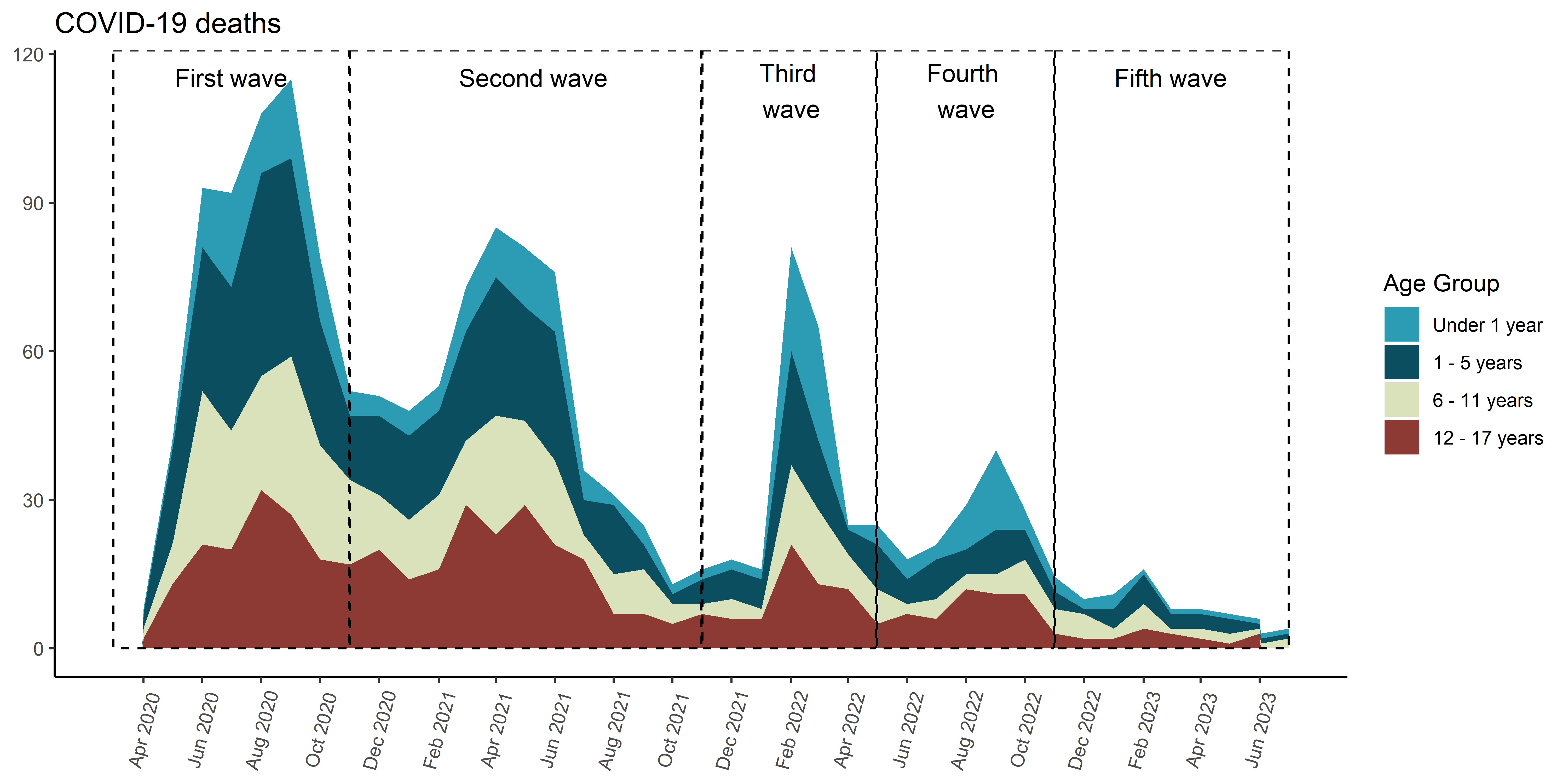
Gráfico de muertes (serie de tiempo) - Menores de 18 años

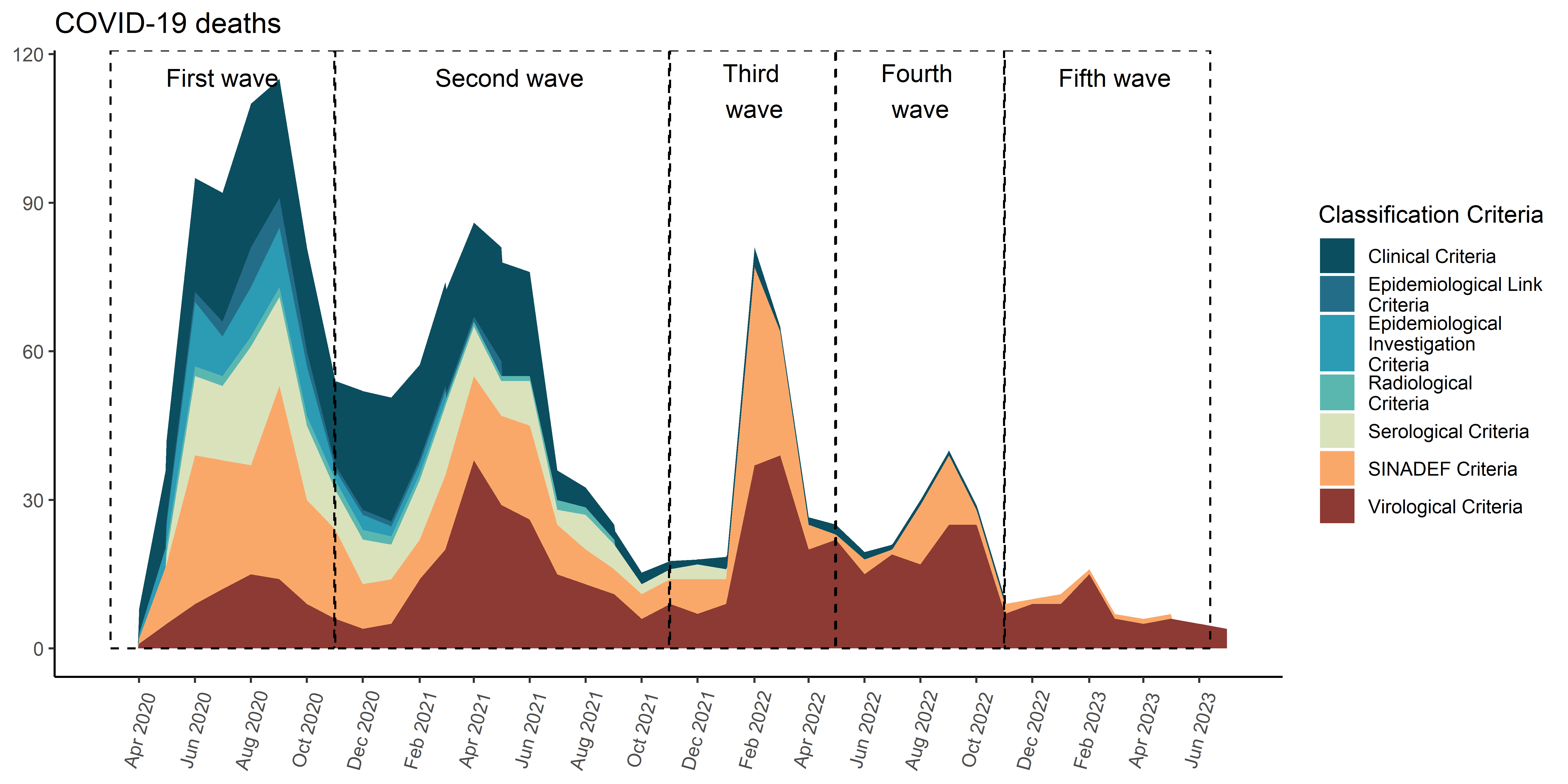
In [139]:

range_fallecidos_und_18 <- fallecidos_total %>%
  summarise(
    min = min(fecha_fallecimiento),
    max = max(fecha_fallecimiento)
  ) %>% 
  collect()

deaths_cases_area <- fallecidos_total %>% 
  count(clasificacion_def, fecha_round) %>% 
  mutate(
    clasificacion_def = case_match(
      clasificacion_def,
      "Criterio serológico" ~ "Serological Criteria",
      "Criterio radiológico" ~ "Radiological Criteria",
      "Criterio SINADEF" ~ "SINADEF Criteria",
      "Criterio virológico" ~ "Virological Criteria",
      "Criterio nexo epidemiológico" ~ "Epidemiological Link Criteria",
      "Criterio clínico" ~ "Clinical Criteria",
      "Criterio investigación Epidemiológica" ~ "Epidemiological Investigation Criteria",
      .default = NA_character_
    )
  ) %>% 
  collect() %>% 
  mutate(
    clasificacion_def = str_wrap(clasificacion_def,
                                 20)
  ) |> 
  ggplot(
    aes(
      x = fecha_round,
      y = n,
      fill = clasificacion_def
    )
  ) +
  geom_area(position = 'stack') +
  innovar::scale_fill_innova("jama") +
  # scale_x_date(
  #   limits = c(ymd("2020-03-01"), ymd("2023-10-31")),
  #   breaks = scales::date_breaks("2 month"), # Cambiar a "6 months" para menos frecuencia
  #   labels = scales::date_format("%b %Y") # Formato de fecha, %b es la abreviatura de mes, %Y es el año
  # ) + 
  scale_x_date(
    limits = c(ymd("2020-03-01"), ymd("2023-07-01")),
    breaks = seq(from = ceiling_date(ymd("2020-03-01"), "month"),
                 to = floor_date(ymd("2023-07-01"), "month"),
                 by = "2 months"), 
    # date_breaks = "2 month",
    date_labels = "%b %Y"
  ) +
  labs(
    y = NULL,
    x = NULL,
    title = "COVID-19 deaths",
    fill = "Classification Criteria"
  ) + 
  annotate(
    geom = "rect",
    xmin = as.Date("2020-03-01"), 
    xmax = as.Date("2020-10-31"), 
    ymin = 0, # El rectángulo se extiende hasta la parte inferior del gráfico
    ymax = Inf, # El rectángulo se extiende hasta la parte superior del gráfico
    color = "black", # Color de la línea
    fill = NA, # Sin relleno
    linetype = "dashed", # Tipo de línea discontinua
    linewidth = 0.5 # Grosor de la línea
  ) + 
  annotate(
    geom = "text", 
    x = as.Date("2020-07-01"), # Punto medio aproximado de la Ola 2
    y = Inf, # Posición vertical del texto
    label = "First wave", 
    color = "black",
    size = 4, # Tamaño del texto
    vjust = 2 # Ajuste vertical para colocar el texto encima del rectángulo
  ) +
  annotate(
    geom = "rect",
    xmin = as.Date("2020-11-01"), 
    xmax = as.Date("2021-10-31"), 
    ymin = 0, # El rectángulo se extiende hasta la parte inferior del gráfico
    ymax = Inf, # El rectángulo se extiende hasta la parte superior del gráfico
    color = "black", # Color de la línea
    fill = NA, # Sin relleno
    linetype = "dashed", # Tipo de línea discontinua
    linewidth = 0.5 # Grosor de la línea
  ) + 
  annotate(
    geom = "text", 
    x = as.Date("2021-05-10"), # Punto medio aproximado de la Ola 2
    y = Inf, # Posición vertical del texto
    label = "Second wave", 
    color = "black",
    size = 4, # Tamaño del texto
    vjust = 2 # Ajuste vertical para colocar el texto encima del rectángulo
  ) + 
  annotate(
    geom = "rect",
    xmin = as.Date("2021-11-01"), 
    xmax = as.Date("2022-04-30"), 
    ymin = 0, # El rectángulo se extiende hasta la parte inferior del gráfico
    ymax = Inf, # El rectángulo se extiende hasta la parte superior del gráfico
    color = "black", # Color de la línea
    fill = NA, # Sin relleno
    linetype = "dashed", # Tipo de línea discontinua
    linewidth = 0.5 # Grosor de la línea
  ) + 
    annotate(
    geom = "text", 
    x = as.Date("2022-02-01"), # Punto medio aproximado de la Ola 2
    y = Inf, # Posición vertical del texto
    label = "Third \nwave", 
    color = "black",
    size = 4, # Tamaño del texto
    vjust = 1.25 # Ajuste vertical para colocar el texto encima del rectángulo
  ) + 
  annotate(
    geom = "rect",
    xmin = as.Date("2022-05-01"), 
    xmax = as.Date("2022-10-31"), 
    ymin = 0, # El rectángulo se extiende hasta la parte inferior del gráfico
    ymax = Inf, # El rectángulo se extiende hasta la parte superior del gráfico
    color = "black", # Color de la línea
    fill = NA, # Sin relleno
    linetype = "dashed", # Tipo de línea discontinua
    linewidth = 0.5 # Grosor de la línea
  ) + 
  annotate(
    geom = "text", 
    x = as.Date("2022-08-01"), # Punto medio aproximado de la Ola 2
    y = Inf, # Posición vertical del texto
    label = "Fourth \nwave", 
    color = "black",
    size = 4, # Tamaño del texto
    vjust = 1.25 # Ajuste vertical para colocar el texto encima del rectángulo
  ) +
  annotate(
    geom = "rect",
    xmin = as.Date("2022-11-01"), 
    xmax = range_fallecidos_und_18$max, 
    ymin = 0, # El rectángulo se extiende hasta la parte inferior del gráfico
    ymax = Inf, # El rectángulo se extiende hasta la parte superior del gráfico
    color = "black", # Color de la línea
    fill = NA, # Sin relleno
    linetype = "dashed", # Tipo de línea discontinua
    linewidth = 0.5 # Grosor de la línea
  ) + 
  annotate(
    geom = "text", 
    x = as.Date("2023-03-01"), # Punto medio aproximado de la Ola 2
    y = Inf, # Posición vertical del texto
    label = "Fifth wave", 
    color = "black",
    size = 4, # Tamaño del texto
    vjust = 2 # Ajuste vertical para colocar el texto encima del rectángulo
  ) +
  theme_classic() +
  theme(
    axis.text.x = element_text(
      angle = 75,
      vjust = 0.5
    ),
    axis.ticks.x = element_line()
  ) 

deaths_cases_area

Gráfico de muertes (serie de tiempo) - Grupo Etáreo

In [140]:

deaths_cases_by_age_area <- fallecidos_total %>%
  count(grupo_edad, fecha_round) %>% 
  collect() %>% 
  ggplot(
    aes(
      x = fecha_round,
      y = n,
      fill = grupo_edad
    )
  ) +
  geom_area(position = 'stack') +
  scale_fill_manual(
    values = c("#2C9BB4", "#0B4E60", "#DAE2BC", "#8C3A33")
  ) +
  # scale_x_date(
  #   limits = c(ymd("2020-03-01"), ymd("2023-10-31")),
  #   breaks = scales::date_breaks("2 month"), # Cambiar a "6 months" para menos frecuencia
  #   labels = scales::date_format("%b %Y") # Formato de fecha, %b es la abreviatura de mes, %Y es el año
  # ) + 
  scale_x_date(
    limits = c(ymd("2020-03-01"), ymd("2023-07-01")),
    breaks = seq(from = ceiling_date(ymd("2020-03-01"), "month"),
                 to = floor_date(ymd("2023-07-01"), "month"),
                 by = "2 months"), 
    # date_breaks = "2 month",
    date_labels = "%b %Y"
  ) +
  labs(
    y = NULL,
    x = NULL,
    title = "COVID-19 deaths",
    fill = "Age Group"
  ) + 
  annotate(
    geom = "rect",
    xmin = as.Date("2020-03-01"), 
    xmax = as.Date("2020-10-31"), 
    ymin = 0, # El rectángulo se extiende hasta la parte inferior del gráfico
    ymax = Inf, # El rectángulo se extiende hasta la parte superior del gráfico
    color = "black", # Color de la línea
    fill = NA, # Sin relleno
    linetype = "dashed", # Tipo de línea discontinua
    linewidth = 0.5 # Grosor de la línea
  ) + 
  annotate(
    geom = "text", 
    x = as.Date("2020-07-01"), # Punto medio aproximado de la Ola 2
    y = Inf, # Posición vertical del texto
    label = "First wave", 
    color = "black",
    size = 4, # Tamaño del texto
    vjust = 2 # Ajuste vertical para colocar el texto encima del rectángulo
  ) +
  annotate(
    geom = "rect",
    xmin = as.Date("2020-11-01"), 
    xmax = as.Date("2021-10-31"), 
    ymin = 0, # El rectángulo se extiende hasta la parte inferior del gráfico
    ymax = Inf, # El rectángulo se extiende hasta la parte superior del gráfico
    color = "black", # Color de la línea
    fill = NA, # Sin relleno
    linetype = "dashed", # Tipo de línea discontinua
    linewidth = 0.5 # Grosor de la línea
  ) + 
  annotate(
    geom = "text", 
    x = as.Date("2021-05-10"), # Punto medio aproximado de la Ola 2
    y = Inf, # Posición vertical del texto
    label = "Second wave", 
    color = "black",
    size = 4, # Tamaño del texto
    vjust = 2 # Ajuste vertical para colocar el texto encima del rectángulo
  ) + 
  annotate(
    geom = "rect",
    xmin = as.Date("2021-11-01"), 
    xmax = as.Date("2022-04-30"), 
    ymin = 0, # El rectángulo se extiende hasta la parte inferior del gráfico
    ymax = Inf, # El rectángulo se extiende hasta la parte superior del gráfico
    color = "black", # Color de la línea
    fill = NA, # Sin relleno
    linetype = "dashed", # Tipo de línea discontinua
    linewidth = 0.5 # Grosor de la línea
  ) + 
    annotate(
    geom = "text", 
    x = as.Date("2022-02-01"), # Punto medio aproximado de la Ola 2
    y = Inf, # Posición vertical del texto
    label = "Third \nwave", 
    color = "black",
    size = 4, # Tamaño del texto
    vjust = 1.25 # Ajuste vertical para colocar el texto encima del rectángulo
  ) + 
  annotate(
    geom = "rect",
    xmin = as.Date("2022-05-01"), 
    xmax = as.Date("2022-10-31"), 
    ymin = 0, # El rectángulo se extiende hasta la parte inferior del gráfico
    ymax = Inf, # El rectángulo se extiende hasta la parte superior del gráfico
    color = "black", # Color de la línea
    fill = NA, # Sin relleno
    linetype = "dashed", # Tipo de línea discontinua
    linewidth = 0.5 # Grosor de la línea
  ) + 
  annotate(
    geom = "text", 
    x = as.Date("2022-08-01"), # Punto medio aproximado de la Ola 2
    y = Inf, # Posición vertical del texto
    label = "Fourth \nwave", 
    color = "black",
    size = 4, # Tamaño del texto
    vjust = 1.25 # Ajuste vertical para colocar el texto encima del rectángulo
  ) +
  annotate(
    geom = "rect",
    xmin = as.Date("2022-11-01"), 
    xmax = as.Date("2023-07-01"), 
    ymin = 0, # El rectángulo se extiende hasta la parte inferior del gráfico
    ymax = Inf, # El rectángulo se extiende hasta la parte superior del gráfico
    color = "black", # Color de la línea
    fill = NA, # Sin relleno
    linetype = "dashed", # Tipo de línea discontinua
    linewidth = 0.5 # Grosor de la línea
  ) + 
  annotate(
    geom = "text", 
    x = as.Date("2023-03-01"),
    y = Inf, # Posición vertical del texto
    label = "Fifth wave", 
    color = "black",
    size = 4, # Tamaño del texto
    vjust = 2 # Ajuste vertical para colocar el texto encima del rectángulo
  ) +
  theme_classic() +
  theme(
    axis.text.x = element_text(
      angle = 75,
      vjust = 0.5
    ),
    axis.ticks.x = element_line()
  ) 

deaths_cases_by_age_area

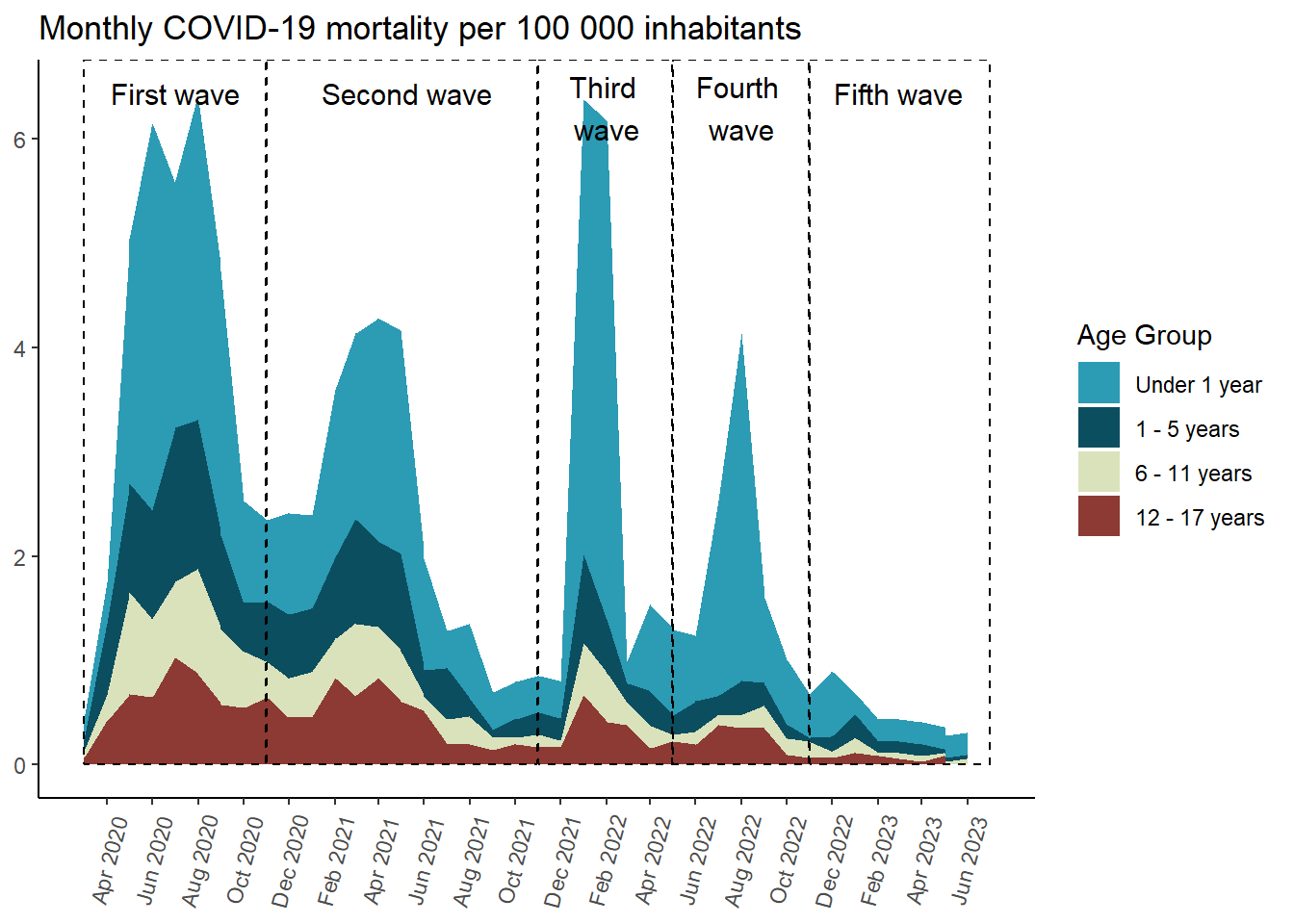
Gráfico Mortalidad (serie de tiempo)

In [141]:

mortality_cases_by_age_area <- results_per_month_mortalidad$grupo_edad$index %>% 
  mutate(
    time = make_date(anio, mes, "1")
  ) %>% 
  ggplot(
    aes(
      x = time,
      y = rate,
      fill = grupo_edad
    )
  ) +
  geom_area(position = 'stack') +
  scale_fill_manual(
    values = c("#2C9BB4", "#0B4E60", "#DAE2BC", "#8C3A33")
  ) +
  scale_x_date(
    limits = c(ymd("2020-03-01"), ymd("2023-07-01")),
    breaks = seq(from = ceiling_date(ymd("2020-03-01"), "month"),
                 to = floor_date(ymd("2023-07-01"), "month"),
                 by = "2 months"), 
    # date_breaks = "2 month",
    date_labels = "%b %Y"
  ) +
  labs(
    y = NULL,
    x = NULL,
    title = "Monthly COVID-19 mortality per 100 000 inhabitants",
    fill = "Age Group"
  ) + 
  annotate(
    geom = "rect",
    xmin = as.Date("2020-03-01"), 
    xmax = as.Date("2020-10-31"), 
    ymin = 0, # El rectángulo se extiende hasta la parte inferior del gráfico
    ymax = Inf, # El rectángulo se extiende hasta la parte superior del gráfico
    color = "black", # Color de la línea
    fill = NA, # Sin relleno
    linetype = "dashed", # Tipo de línea discontinua
    linewidth = 0.5 # Grosor de la línea
  ) + 
  annotate(
    geom = "text", 
    x = as.Date("2020-07-01"), # Punto medio aproximado de la Ola 2
    y = Inf, # Posición vertical del texto
    label = "First wave", 
    color = "black",
    size = 4, # Tamaño del texto
    vjust = 2 # Ajuste vertical para colocar el texto encima del rectángulo
  ) +
  annotate(
    geom = "rect",
    xmin = as.Date("2020-11-01"), 
    xmax = as.Date("2021-10-31"), 
    ymin = 0, # El rectángulo se extiende hasta la parte inferior del gráfico
    ymax = Inf, # El rectángulo se extiende hasta la parte superior del gráfico
    color = "black", # Color de la línea
    fill = NA, # Sin relleno
    linetype = "dashed", # Tipo de línea discontinua
    linewidth = 0.5 # Grosor de la línea
  ) + 
  annotate(
    geom = "text", 
    x = as.Date("2021-05-10"), # Punto medio aproximado de la Ola 2
    y = Inf, # Posición vertical del texto
    label = "Second wave", 
    color = "black",
    size = 4, # Tamaño del texto
    vjust = 2 # Ajuste vertical para colocar el texto encima del rectángulo
  ) + 
  annotate(
    geom = "rect",
    xmin = as.Date("2021-11-01"), 
    xmax = as.Date("2022-04-30"), 
    ymin = 0, # El rectángulo se extiende hasta la parte inferior del gráfico
    ymax = Inf, # El rectángulo se extiende hasta la parte superior del gráfico
    color = "black", # Color de la línea
    fill = NA, # Sin relleno
    linetype = "dashed", # Tipo de línea discontinua
    linewidth = 0.5 # Grosor de la línea
  ) + 
    annotate(
    geom = "text", 
    x = as.Date("2022-02-01"), # Punto medio aproximado de la Ola 2
    y = Inf, # Posición vertical del texto
    label = "Third \nwave", 
    color = "black",
    size = 4, # Tamaño del texto
    vjust = 1.25 # Ajuste vertical para colocar el texto encima del rectángulo
  ) + 
  annotate(
    geom = "rect",
    xmin = as.Date("2022-05-01"), 
    xmax = as.Date("2022-10-31"), 
    ymin = 0, # El rectángulo se extiende hasta la parte inferior del gráfico
    ymax = Inf, # El rectángulo se extiende hasta la parte superior del gráfico
    color = "black", # Color de la línea
    fill = NA, # Sin relleno
    linetype = "dashed", # Tipo de línea discontinua
    linewidth = 0.5 # Grosor de la línea
  ) + 
  annotate(
    geom = "text", 
    x = as.Date("2022-08-01"), # Punto medio aproximado de la Ola 2
    y = Inf, # Posición vertical del texto
    label = "Fourth \nwave", 
    color = "black",
    size = 4, # Tamaño del texto
    vjust = 1.25 # Ajuste vertical para colocar el texto encima del rectángulo
  ) +
  annotate(
    geom = "rect",
    xmin = as.Date("2022-11-01"), 
    xmax = as.Date("2023-07-01"), 
    ymin = 0, # El rectángulo se extiende hasta la parte inferior del gráfico
    ymax = Inf, # El rectángulo se extiende hasta la parte superior del gráfico
    color = "black", # Color de la línea
    fill = NA, # Sin relleno
    linetype = "dashed", # Tipo de línea discontinua
    linewidth = 0.5 # Grosor de la línea
  ) + 
  annotate(
    geom = "text", 
    x = as.Date("2023-03-01"),
    y = Inf, # Posición vertical del texto
    label = "Fifth wave", 
    color = "black",
    size = 4, # Tamaño del texto
    vjust = 2 # Ajuste vertical para colocar el texto encima del rectángulo
  ) +
  theme_classic() +
  theme(
    axis.text.x = element_text(
      angle = 75,
      vjust = 0.5
    ),
    axis.ticks.x = element_line()
  ) 

mortality_cases_by_age_area

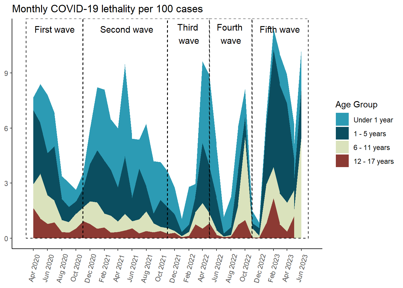
Gráfico Letalidad (serie de tiempo)

No se está mostrando en la gráfica la información de marzo de 2020, debido a la enorme diferencia entre su valor de letalidad con respecto al resto de letalidades.

In [142]:

results_per_month_letalidad$grupo_edad$index |> 
  slice(1:8) |> 
  mutate(rate = round(rate, 3)) |> 
  gt::gt()

anio	mes	grupo_edad	rate
2020	3	Under 1 year	25.000
2020	3	1 - 5 years	33.333
2020	3	6 - 11 years	15.385
2020	3	12 - 17 years	9.091
2020	4	Under 1 year	0.697
2020	4	1 - 5 years	4.017
2020	4	6 - 11 years	1.322
2020	4	12 - 17 years	1.635

In [143]:

lethality_cases_by_age_area <- results_per_month_letalidad$grupo_edad$index %>% 
  mutate(
    time = make_date(anio, mes, "1")
  ) %>% 
  filter(
    time > ymd("2020-03-01")
  ) |> 
  ggplot(
    aes(
      x = time,
      y = rate,
      fill = grupo_edad
    )
  ) +
  geom_area(position = 'stack') +
  scale_fill_manual(
    values = c("#2C9BB4", "#0B4E60", "#DAE2BC", "#8C3A33")
  ) +
  scale_x_date(
    limits = c(ymd("2020-03-01"), ymd("2023-07-01")),
    breaks = seq(from = ceiling_date(ymd("2020-03-01"), "month"),
                 to = floor_date(ymd("2023-07-01"), "month"),
                 by = "2 months"), 
    # date_breaks = "2 month",
    date_labels = "%b %Y"
  ) +
  labs(
    y = NULL,
    x = NULL,
    title = "Monthly COVID-19 lethality per 100 cases",
    fill = "Age Group"
  ) + 
  annotate(
    geom = "rect",
    xmin = as.Date("2020-03-01"), 
    xmax = as.Date("2020-10-31"), 
    ymin = 0, # El rectángulo se extiende hasta la parte inferior del gráfico
    ymax = Inf, # El rectángulo se extiende hasta la parte superior del gráfico
    color = "black", # Color de la línea
    fill = NA, # Sin relleno
    linetype = "dashed", # Tipo de línea discontinua
    linewidth = 0.5 # Grosor de la línea
  ) + 
  annotate(
    geom = "text", 
    x = as.Date("2020-07-01"), # Punto medio aproximado de la Ola 2
    y = Inf, # Posición vertical del texto
    label = "First wave", 
    color = "black",
    size = 4, # Tamaño del texto
    vjust = 2 # Ajuste vertical para colocar el texto encima del rectángulo
  ) +
  annotate(
    geom = "rect",
    xmin = as.Date("2020-11-01"), 
    xmax = as.Date("2021-10-31"), 
    ymin = 0, # El rectángulo se extiende hasta la parte inferior del gráfico
    ymax = Inf, # El rectángulo se extiende hasta la parte superior del gráfico
    color = "black", # Color de la línea
    fill = NA, # Sin relleno
    linetype = "dashed", # Tipo de línea discontinua
    linewidth = 0.5 # Grosor de la línea
  ) + 
  annotate(
    geom = "text", 
    x = as.Date("2021-05-10"), # Punto medio aproximado de la Ola 2
    y = Inf, # Posición vertical del texto
    label = "Second wave", 
    color = "black",
    size = 4, # Tamaño del texto
    vjust = 2 # Ajuste vertical para colocar el texto encima del rectángulo
  ) + 
  annotate(
    geom = "rect",
    xmin = as.Date("2021-11-01"), 
    xmax = as.Date("2022-04-30"), 
    ymin = 0, # El rectángulo se extiende hasta la parte inferior del gráfico
    ymax = Inf, # El rectángulo se extiende hasta la parte superior del gráfico
    color = "black", # Color de la línea
    fill = NA, # Sin relleno
    linetype = "dashed", # Tipo de línea discontinua
    linewidth = 0.5 # Grosor de la línea
  ) + 
    annotate(
    geom = "text", 
    x = as.Date("2022-02-01"), # Punto medio aproximado de la Ola 2
    y = Inf, # Posición vertical del texto
    label = "Third \nwave", 
    color = "black",
    size = 4, # Tamaño del texto
    vjust = 1.25 # Ajuste vertical para colocar el texto encima del rectángulo
  ) + 
  annotate(
    geom = "rect",
    xmin = as.Date("2022-05-01"), 
    xmax = as.Date("2022-10-31"), 
    ymin = 0, # El rectángulo se extiende hasta la parte inferior del gráfico
    ymax = Inf, # El rectángulo se extiende hasta la parte superior del gráfico
    color = "black", # Color de la línea
    fill = NA, # Sin relleno
    linetype = "dashed", # Tipo de línea discontinua
    linewidth = 0.5 # Grosor de la línea
  ) + 
  annotate(
    geom = "text", 
    x = as.Date("2022-08-01"), # Punto medio aproximado de la Ola 2
    y = Inf, # Posición vertical del texto
    label = "Fourth \nwave", 
    color = "black",
    size = 4, # Tamaño del texto
    vjust = 1.25 # Ajuste vertical para colocar el texto encima del rectángulo
  ) +
  annotate(
    geom = "rect",
    xmin = as.Date("2022-11-01"), 
    xmax = as.Date("2023-07-01"), 
    ymin = 0, # El rectángulo se extiende hasta la parte inferior del gráfico
    ymax = Inf, # El rectángulo se extiende hasta la parte superior del gráfico
    color = "black", # Color de la línea
    fill = NA, # Sin relleno
    linetype = "dashed", # Tipo de línea discontinua
    linewidth = 0.5 # Grosor de la línea
  ) + 
  annotate(
    geom = "text", 
    x = as.Date("2023-03-01"),
    y = Inf, # Posición vertical del texto
    label = "Fifth wave", 
    color = "black",
    size = 4, # Tamaño del texto
    vjust = 2 # Ajuste vertical para colocar el texto encima del rectángulo
  ) +
  theme_classic() +
  theme(
    axis.text.x = element_text(
      angle = 75,
      vjust = 0.5
    ),
    axis.ticks.x = element_line()
  ) 

lethality_cases_by_age_area

Pirámide frecuencia - Edades

In [144]:

fallecidos_total_df %>% 
  mutate(
    edad_declarada = factor(edad_declarada)
  ) %>% 
  age_pyramid(
    age_group = "edad_declarada",
    split_by = "sexo"
  ) +
  scale_fill_brewer(palette = "Dark2") +
  labs(
    x = "Age",
    fill = "Sex",
    y = "Frequency"
  ) +
  theme_classic()

Scale for fill is already present.
Adding another scale for fill, which will replace the existing scale.

In [145]:

fallecidos_total_df %>% 
  age_pyramid(
    age_group = "grupo_edad",
    split_by = "sexo"
  ) +
  scale_fill_brewer(palette = "Dark2") +
  labs(
    x = "Age Group",
    fill = "Sex",
    y = "Frequency"
  ) +
  theme_classic()

Scale for fill is already present.
Adding another scale for fill, which will replace the existing scale.

Pirámide proporcional - Edades

In [146]:

fallecidos_total_df %>% 
  mutate(
    edad_declarada = factor(edad_declarada)
  ) %>% 
  age_pyramid(
    age_group = "edad_declarada",
    split_by = "sexo",
    proportional = TRUE
  ) +
   scale_fill_brewer(palette = "Dark2") +
  labs(
    x = "Age",
    fill = "Sex",
    y = "Percentage"
  ) +
  theme_classic()

Scale for fill is already present.
Adding another scale for fill, which will replace the existing scale.

In [147]:

fallecidos_total_df %>% 
  age_pyramid(
    age_group = "grupo_edad",
    split_by = "sexo",
    proportional = TRUE
  ) +
   scale_fill_brewer(palette = "Dark2") +
  labs(
    x = "Age Group",
    fill = "Sex",
    y = "Percentage"
  ) +
  theme_classic()

Scale for fill is already present.
Adding another scale for fill, which will replace the existing scale.

Departamento

In [148]:

fallecidos_dep_100k_sf <- peru_dep_sf %>%
  rename(departamento = dep) %>% 
  left_join(
    results_mortalidad$departamento$index
  ) %>%
  ungroup()

Joining with `by = join_by(departamento)`

In [149]:

fallecidos_dep_100k_map <- fallecidos_dep_100k_sf %>%
  ggplot() +
  geom_sf(aes(fill = rate)) +
  guides(
    fill = guide_legend(
      str_wrap("Mean monthly COVID-19 mortality per 100 000 inhabitants",
               20)
    )
  ) +
  scale_fill_distiller(palette = "Oranges", # Old: YlOrBr
                       direction = 1) + 
  theme_void()

fallecidos_dep_100k_map

Figura 21: Mortalidad COVID-19 por 100K habitantes de acuerdo al departamento (14-03-2020 a 13-06-2023)

In [150]:

In [151]:

tbl_summ_mort_dep_pre <- results_mortalidad$departamento$index %>% 
  mutate(
    rate = formattable::digits(rate, 3)
  ) %>% 
  mutate(
    departamento = str_to_title(departamento)
  ) 

tbl_summ_mort_dep <- tbl_summ_mort_dep_pre %>% 
  rename_with(
    .fn = ~ paste0("**", str_to_title(.x), "**")
  ) %>% 
  gt::gt() %>% 
  gt::cols_label(
    .fn = gt::md,
    .process_units = TRUE
  )

tbl_summ_mort_dep

Tabla 19: Mortalidad COVID-19 por 100K habitantes de acuerdo al departamento (07-03-2020 a 17-06-2023)

Departamento	Rate
Amazonas	1.018
Ancash	0.470
Apurimac	0.955
Arequipa	0.521
Ayacucho	0.534
Cajamarca	0.437
Callao	0.775
Cusco	0.552
Huancavelica	1.110
Huanuco	0.598
Ica	0.805
Junin	0.606
La Libertad	0.425
Lambayeque	0.831
Lima	0.465
Loreto	0.716
Madre De Dios	2.599
Moquegua	2.099
Pasco	1.457
Piura	0.662
Puno	0.641
San Martin	0.610
Tacna	1.519
Tumbes	1.710
Ucayali	2.335

In [152]:

tbl_summ_mort_dep_pre %>% 
  rename_with(
    .fn = str_to_title
  ) %>% 
  huxtable::as_hux() %>% 
  huxtable::set_bold(1, 1:2) %>% 
  huxtable::quick_xlsx(file = "02_output/tables/mortalidad_departamento.xlsx",
                       open = FALSE)

tbl_summ_mort_dep %>%
  gt::gtsave("02_output/tables/mortalidad_departamento.docx")

In [153]:

downloadthis::download_file(
  path = "02_output/tables/mortalidad_departamento.xlsx",
  button_label = "Descargar tabla en Excel",
  button_type = "success",
  has_icon = TRUE,
  icon = "fa fa-save"
)

In [154]:

downloadthis::download_file(
  path = "02_output/tables/mortalidad_departamento.docx",
  button_label = "Descargar tabla en Word",
  button_type = "primary",
  has_icon = TRUE,
  icon = "fa fa-save"
)

Departamento y sexo

In [155]:

mortalidad_dep_sex_100k_sf <- peru_dep_sf %>% 
  rename(departamento = dep) %>% 
  inner_join(
    results_mortalidad$departamento_sexo$index
  )

Joining with `by = join_by(departamento)`

In [156]:

mortalidad_dep_sex_100k_sf %>%
  ggplot() +
  geom_sf(aes(fill = rate)) +
  guides(
    fill = guide_legend(
      str_wrap("Mean monthly COVID-19 mortality per 100 000 inhabitants",
               20)
    )
  ) +
  scale_fill_distiller(palette = "Oranges", # Old: "YlOrBr"
                       direction = 1) + 
  facet_wrap(vars(sexo)) + 
  theme_void()

Figura 22: Mortalidad COVID-19 por 100K habitantes de acuerdo al departamento y sexo (14-03-2020 a 13-06-2023)

In [157]:

In [158]:

tbl_summ_mort_dep_sex_pre <- results_mortalidad$departamento_sexo$index %>% 
  mutate(
    rate = formattable::digits(rate, 3),
    departamento = str_to_title(departamento)
  ) %>% 
  pivot_wider(
    names_from = sexo, 
    values_from = rate
  )


tbl_summ_mort_dep_sex <- tbl_summ_mort_dep_sex_pre %>% 
  rename_with(
    .fn = ~ paste0("**", str_to_title(.x), "**")
  ) %>% 
  gt::gt() %>% 
  gt::cols_label(
    .fn = gt::md,
    .process_units = TRUE
  )

tbl_summ_mort_dep_sex

Tabla 20: Mortalidad COVID-19 por 100K habitantes de acuerdo al departamento (14-03-2020 a 13-06-2023)

Departamento	Female	Male
Amazonas	1.692	1.371
Ancash	0.619	0.757
Apurimac	1.586	1.281
Arequipa	0.833	0.827
Ayacucho	1.074	0.915
Cajamarca	0.573	0.631
Callao	0.991	1.122
Cusco	0.698	0.767
Huancavelica	1.353	1.916
Huanuco	0.821	0.926
Ica	1.115	1.170
Junin	0.758	0.869
La Libertad	0.670	0.585
Lambayeque	0.986	1.203
Lima	0.467	0.524
Loreto	0.889	1.035
Madre De Dios	4.496	4.207
Moquegua	4.329	4.163
Pasco	2.594	2.841
Piura	0.797	0.827
Puno	1.036	0.772
San Martin	0.960	0.940
Tacna	3.037	2.526
Tumbes	3.753	2.597
Ucayali	3.125	2.848

In [159]:

tbl_summ_mort_dep_sex_pre %>% 
  rename_with(
    .fn = str_to_title
  ) %>% 
  huxtable::as_hux() %>% 
  huxtable::set_bold(1, 1:3) %>% 
  huxtable::quick_xlsx(file = "02_output/tables/mortalidad_departamento_sexo.xlsx",
                       open = FALSE)

tbl_summ_mort_dep_sex %>%
  gt::gtsave("02_output/tables/mortalidad_departamento_sexo.docx")

In [160]:

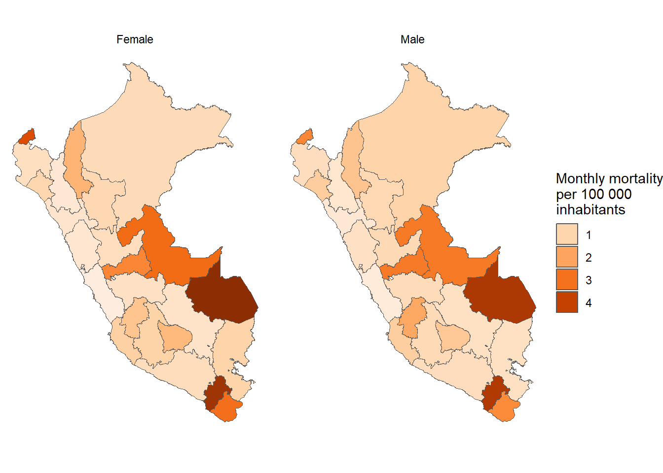
downloadthis::download_file(
  path = "02_output/tables/mortalidad_departamento_sexo.xlsx",
  button_label = "Descargar tabla en Excel",
  button_type = "success",
  has_icon = TRUE,
  icon = "fa fa-save"
)

In [161]:

downloadthis::download_file(
  path = "02_output/tables/mortalidad_departamento_sexo.docx",
  button_label = "Descargar tabla en Word",
  button_type = "primary",
  has_icon = TRUE,
  icon = "fa fa-save"
)

Departamento y edad

In [162]:

mortalidad_dep_edad_100k_sf <- peru_dep_sf %>% 
  rename(departamento = dep) %>% 
  inner_join(
    results_mortalidad$departamento_grupo_edad$index
  )

Joining with `by = join_by(departamento)`

In [163]:

mortalidad_dep_edad_100k_sf %>%
  ggplot() +
  geom_sf(aes(fill = rate)) +
  guides(
    fill = guide_legend(
      str_wrap("Mean monthly COVID-19 mortality per 100 000 inhabitants",
               20)
    )
  ) +
  scale_fill_distiller(palette = "YlOrBr",
                       direction = 1) + 
  facet_wrap(vars(grupo_edad), nrow = 1) + 
  theme_void()

Figura 23: Mortalidad COVID-19 por 100K habitantes de acuerdo al departamento y grupo de edad (14-03-2020 a 13-06-2023)

In [164]:

In [165]:

tbl_summ_mort_dep_edad_pre <- results_mortalidad$departamento_grupo_edad$index %>% 
  mutate(
    rate = formattable::digits(rate, 3),
    departamento = str_to_title(departamento)
  ) %>% 
  pivot_wider(
    names_from = grupo_edad, 
    values_from = rate
  )


tbl_summ_mort_dep_edad <- tbl_summ_mort_dep_edad_pre %>% 
  rename_with(
    .fn = ~ paste0("**", str_to_title(.x), "**")
  ) %>% 
  gt::gt() %>% 
  gt::cols_label(
    .fn = gt::md,
    .process_units = TRUE
  )

tbl_summ_mort_dep_edad

Tabla 21: Mortalidad COVID-19 por 100K habitantes de acuerdo al departamento y grupo de edad(14-03-2020 a 13-06-2023)

Departamento	Under 1 Year	1 - 5 Years	6 - 11 Years	12 - 17 Years
Amazonas	11.234	2.223	2.408	2.673
Ancash	5.072	1.272	0.876	0.952
Apurimac	12.428	3.131	1.776	2.317
Arequipa	6.678	1.082	0.978	1.198
Ayacucho	8.207	1.527	1.241	1.221
Cajamarca	5.587	0.772	0.662	0.757
Callao	7.197	1.412	1.267	1.480
Cusco	5.216	1.235	0.914	0.756
Huancavelica	12.845	3.703	2.122	2.469
Huanuco	7.352	1.739	1.092	1.341
Ica	9.803	1.789	1.204	1.225
Junin	4.985	1.114	0.817	0.802
La Libertad	4.217	0.809	0.775	0.800
Lambayeque	7.289	1.560	1.111	1.046
Lima	2.095	0.553	0.416	0.468
Loreto	4.486	1.198	0.950	1.401
Madre De Dios	45.537	6.442	5.939	6.484
Moquegua	43.234	7.552	6.114	6.429
Pasco	22.171	3.716	3.976	3.763
Piura	4.540	1.269	0.792	0.792
Puno	9.375	1.140	0.905	1.077
San Martin	5.910	1.618	1.118	1.165
Tacna	27.020	NA	3.144	3.646
Tumbes	NA	4.526	5.350	4.038
Ucayali	9.795	4.613	3.602	2.112

In [166]:

tbl_summ_mort_dep_edad_pre %>% 
  rename_with(
    .fn = str_to_title
  ) %>% 
  huxtable::as_hux() %>% 
  huxtable::set_bold(1, 1:5) %>% 
  huxtable::quick_xlsx(file = "02_output/tables/mortalidad_departamento_edad.xlsx",
                       open = FALSE)

tbl_summ_mort_dep_edad %>%
  gt::gtsave("02_output/tables/mortalidad_departamento_edad.docx")

In [167]:

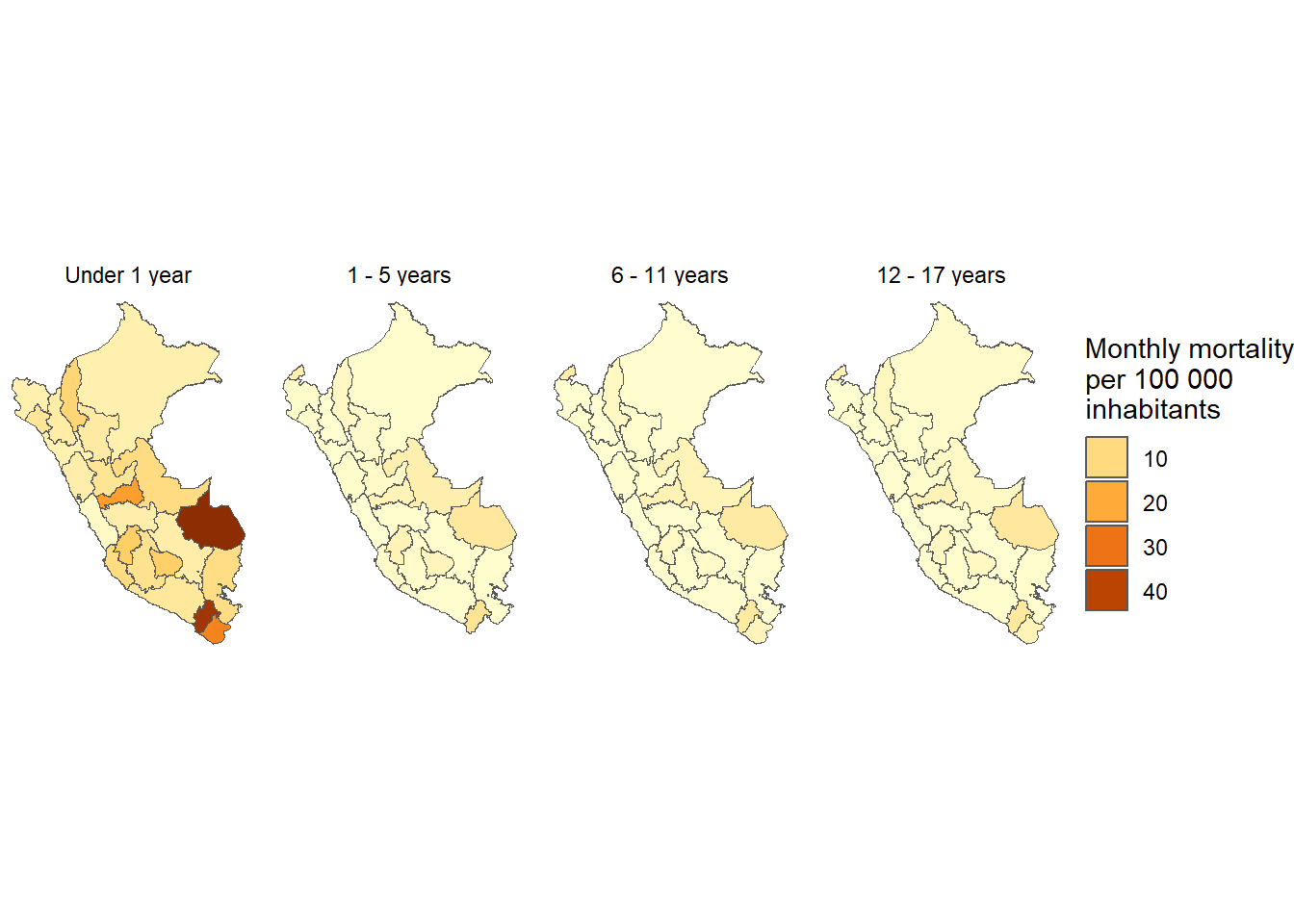
downloadthis::download_file(
  path = "02_output/tables/mortalidad_departamento_edad.xlsx",
  button_label = "Descargar tabla en Excel",
  button_type = "success",
  has_icon = TRUE,
  icon = "fa fa-save"
)

In [168]:

downloadthis::download_file(
  path = "02_output/tables/mortalidad_departamento_edad.docx",
  button_label = "Descargar tabla en Word",
  button_type = "primary",
  has_icon = TRUE,
  icon = "fa fa-save"
)

Departamento y olas

In [169]:

mortalidad_dep_olas_mother <- crossing(
  ola_covid = levels(results_mortalidad$departamento_ola_covid$index$ola_covid),
  departamento = unique(results_mortalidad$departamento_ola_covid$index$departamento)
)

mortalidad_dep_olas_100k <- mortalidad_dep_olas_mother %>% 
  left_join(results_mortalidad$departamento_ola_covid$index) %>% 
  bind_rows(
    results_mortalidad$departamento$index %>% 
      mutate(ola_covid = "Overall")
  ) %>% 
  mutate(
    ola_covid = fct_recode(
      ola_covid,
      "1st wave" = "1 (Mar – Oct 2020)",
      "2nd wave" = "2 (Nov 2020 – Oct 2021)",
      "3rd wave" = "3 (Nov 2021 – Apr 2022)",
      "4th wave" = "4 (May 2022 – Oct 2022)",
      "5th wave" = "5 (Nov 2022 – Jun 2023)"
    ),
    ola_covid = fct_relevel(ola_covid,
                            "Overall")
  ) %>% 
  arrange(ola_covid)

Joining with `by = join_by(ola_covid, departamento)`

mortalidad_dep_olas_100k_sf <- peru_dep_sf %>%
  rename(departamento = dep) %>% 
  left_join(
    mortalidad_dep_olas_100k
  ) %>%
  ungroup()

Joining with `by = join_by(departamento)`

In [170]:

mortalidad_dep_olas_100k_map <- 
  mortalidad_dep_olas_100k_sf %>%
  ggplot() +
  geom_sf(aes(fill = rate)) +
  guides(
    fill = guide_legend(
      str_wrap("Mean monthly COVID-19 mortality per 100 000 inhabitants",
               20)
    )
  ) +
  # scale_fill_distiller(palette = "YlOrBr",
  #                      direction = 1) + 
  scale_fill_gradientn(
    colors = scales::pal_brewer("seq", "Oranges", 1)(4),
    values = scales::rescale(c(0, 1, 2, 3, max(mortalidad_dep_olas_100k_sf$rate, na.rm = TRUE))),
    breaks = c(0, 1, 2, 3, max(mortalidad_dep_olas_100k_sf$rate, na.rm = TRUE)),
    labels = c("0", "1", "2", "3", "Max"),
    limits = c(0,
               max(mortalidad_dep_olas_100k_sf$rate, na.rm = TRUE)),
    na.value = "white"
  ) +
  facet_wrap(vars(ola_covid), nrow = 1) + 
  theme_void()

mortalidad_dep_olas_100k

# A tibble: 150 × 3
   ola_covid departamento  rate
   <fct>     <chr>        <dbl>
 1 Overall   AMAZONAS     1.02 
 2 Overall   ANCASH       0.470
 3 Overall   APURIMAC     0.955
 4 Overall   AREQUIPA     0.521
 5 Overall   AYACUCHO     0.534
 6 Overall   CAJAMARCA    0.437
 7 Overall   CALLAO       0.775
 8 Overall   CUSCO        0.552
 9 Overall   HUANCAVELICA 1.11 
10 Overall   HUANUCO      0.598
# ℹ 140 more rows

In [171]:

In [172]:

tbl_summ_mort_dep_ola_pre <- mortalidad_dep_olas_100k %>% 
  mutate(
    rate = formattable::digits(rate, 3),
    departamento = str_to_title(departamento)
  ) %>% 
  pivot_wider(
    names_from = ola_covid, 
    values_from = rate
  )


tbl_summ_mort_dep_ola <- tbl_summ_mort_dep_ola_pre %>% 
  rename_with(
    .fn = ~ paste0("**", str_to_title(.x), "**")
  ) %>% 
  gt::gt() %>% 
  gt::cols_label(
    .fn = gt::md,
    .process_units = TRUE
  )

tbl_summ_mort_dep_ola

Tabla 22: Mortalidad COVID-19 por 100K habitantes de acuerdo al departamento y Olas COVID(14-03-2020 a 13-06-2023)

Departamento	Overall	1st Wave	2nd Wave	3rd Wave	4th Wave	5th Wave
Amazonas	1.018	1.511	1.115	0.770	0.604	0.611
Ancash	0.470	0.765	0.381	0.490	0.424	0.278
Apurimac	0.955	0.644	0.970	1.364	0.682	NA
Arequipa	0.521	0.465	0.690	0.450	0.249	0.234
Ayacucho	0.534	0.541	0.482	0.650	0.434	0.459
Cajamarca	0.437	0.469	0.434	0.547	0.393	0.277
Callao	0.775	0.761	0.957	0.695	0.697	0.349
Cusco	0.552	0.879	0.554	0.760	0.228	0.234
Huancavelica	1.110	1.762	0.976	0.918	NA	0.862
Huanuco	0.598	0.704	0.620	0.518	0.363	0.388
Ica	0.805	1.035	0.870	0.351	0.648	0.469
Junin	0.606	0.808	0.552	0.716	0.376	NA
La Libertad	0.425	0.699	0.304	0.545	0.297	0.164
Lambayeque	0.831	1.060	1.100	0.504	0.315	0.239
Lima	0.465	0.939	0.470	0.417	0.282	0.158
Loreto	0.716	1.158	0.668	0.547	0.240	0.227
Madre De Dios	2.599	2.331	3.118	3.580	1.790	NA
Moquegua	2.099	2.117	2.073	2.135	2.135	NA
Pasco	1.457	1.642	1.639	1.135	NA	1.136
Piura	0.662	0.871	0.738	0.430	0.345	NA
Puno	0.641	1.046	0.409	0.821	0.638	0.285
San Martin	0.610	0.776	0.737	0.320	0.630	0.305
Tacna	1.519	2.269	1.276	1.133	NA	NA
Tumbes	1.710	2.108	1.578	1.309	1.309	1.309
Ucayali	2.335	3.874	1.401	NA	0.683	NA

In [173]:

tbl_summ_mort_dep_ola_pre %>% 
  rename_with(
    .fn = str_to_title
  ) %>% 
  huxtable::as_hux() %>% 
  huxtable::set_bold(1, 1:6) %>% 
  huxtable::quick_xlsx(file = "02_output/tables/mortalidad_departamento_ola.xlsx",
                       open = FALSE)

tbl_summ_mort_dep_ola %>%
  gt::gtsave("02_output/tables/mortalidad_departamento_ola.docx")

In [174]:

downloadthis::download_file(
  path = "02_output/tables/mortalidad_departamento_ola.xlsx",
  button_label = "Descargar tabla en Excel",
  button_type = "success",
  has_icon = TRUE,
  icon = "fa fa-save"
)

In [175]:

downloadthis::download_file(
  path = "02_output/tables/mortalidad_departamento_ola.docx",
  button_label = "Descargar tabla en Word",
  button_type = "primary",
  has_icon = TRUE,
  icon = "fa fa-save"
)

Regiones

In [176]:

mortalidad_reg_100k_sf <- peru_reg_sf %>%
  left_join(
    results_mortalidad$region$index
  )

Joining with `by = join_by(region)`

In [177]:

mortalidad_reg_100k_map <- mortalidad_reg_100k_sf %>%
  ggplot() +
  geom_sf(aes(fill = rate)) +
  guides(
    fill = guide_legend(
      str_wrap("Mean monthly COVID-19 mortality per 100 000 inhabitants",
               20)
    )
  ) +
  ggsflabel::geom_sf_label(aes(label = region)) +
  scale_fill_distiller(palette = "Oranges", # Old: YlOrBr
                       direction = 1) + 
  theme_void()

mortalidad_reg_100k_map

Warning in st_point_on_surface.sfc(data$geometry): st_point_on_surface may not
give correct results for longitude/latitude data

Figura 24: Mortalidad COVID-19 por 100K habitantes de acuerdo a la región (14-03-2020 a 13-06-2023)

In [178]:

In [179]:

tbl_summ_mort_reg_pre <- results_mortalidad$region$index %>% 
  mutate(
    rate = formattable::digits(rate, 3)
  )


tbl_summ_mort_reg <- tbl_summ_mort_reg_pre %>% 
  rename_with(
    .fn = ~ paste0("**", str_to_title(.x), "**")
  ) %>% 
  gt::gt() %>% 
  gt::cols_label(
    .fn = gt::md,
    .process_units = TRUE
  )

tbl_summ_mort_reg

Tabla 23: Mortalidad COVID-19 por 100K habitantes de acuerdo a la región(14-03-2020 a 13-06-2023)

Region	Rate
Coast	0.427
Highlands	0.351
Jungle	0.668

In [180]:

tbl_summ_mort_reg_pre %>% 
  rename_with(
    .fn = str_to_title
  ) %>% 
  huxtable::as_hux() %>% 
  huxtable::set_bold(1, 1:2) %>% 
  huxtable::quick_xlsx(file = "02_output/tables/mortalidad_region.xlsx",
                       open = FALSE)

tbl_summ_mort_reg %>%
  gt::gtsave("02_output/tables/mortalidad_region.docx")

In [181]:

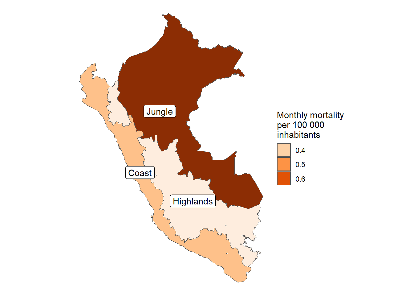
downloadthis::download_file(
  path = "02_output/tables/mortalidad_region.xlsx",
  button_label = "Descargar tabla en Excel",
  button_type = "success",
  has_icon = TRUE,
  icon = "fa fa-save"
)

In [182]:

downloadthis::download_file(
  path = "02_output/tables/mortalidad_region.docx",
  button_label = "Descargar tabla en Word",
  button_type = "primary",
  has_icon = TRUE,
  icon = "fa fa-save"
)

Macrorregiones

In [183]:

mortalidad_macro_100k_sf <- peru_macro_sf %>%
  left_join(
    results_mortalidad$macrorregion$index
  )

Joining with `by = join_by(macrorregion)`

In [184]:

mort_macro_map <- mortalidad_macro_100k_sf %>%
  mutate(
    macrorregion = str_wrap(macrorregion, width = 15)
  ) %>%
  ggplot() +
  geom_sf(aes(fill = rate)) +
  ggsflabel::geom_sf_label_repel(aes(label = macrorregion),
                                 force = 100,
                                 seed = 2024) +
  guides(
    fill = guide_legend(
      str_wrap("Mean monthly COVID-19 mortality per 100 000 inhabitants", 
               20)
    )
  ) +
  scale_fill_distiller(palette = "Oranges", # Old: YlOrBr
                       direction = 1) + 
  theme_void()

mort_macro_map

Warning in st_point_on_surface.sfc(data$geometry): st_point_on_surface may not
give correct results for longitude/latitude data

Figura 25: Mortalidad COVID-19 por 100K habitantes de acuerdo a la macrorregión (14-03-2020 a 13-06-2023)

In [185]:

In [186]:

tbl_summ_mort_macro_pre <- results_mortalidad$macrorregion$index %>% 
  mutate(
    rate = formattable::digits(rate, 3)
  )


tbl_summ_mort_macro <- tbl_summ_mort_macro_pre %>% 
  rename_with(
    .fn = ~ paste0("**", str_to_title(.x), "**")
  ) %>% 
  gt::gt() %>% 
  gt::cols_label(
    .fn = gt::md,
    .process_units = TRUE
  )

tbl_summ_mort_macro

Tabla 24: Mortalidad COVID-19 por 100K habitantes de acuerdo a la macrorregión(14-03-2020 a 13-06-2023)

Macrorregion	Rate
Center	0.363
East	0.644
Metropolitan Lima and Callao	0.466
North	0.430
South	0.418

In [187]:

tbl_summ_mort_macro_pre %>% 
  rename_with(
    .fn = str_to_title
  ) %>% 
  huxtable::as_hux() %>% 
  huxtable::set_bold(1, 1:2) %>% 
  huxtable::quick_xlsx(file = "02_output/tables/mortalidad_macrorregion.xlsx",
                       open = FALSE)

tbl_summ_mort_macro %>%
  gt::gtsave("02_output/tables/mortalidad_departamento_macrorregion.docx")

In [188]:

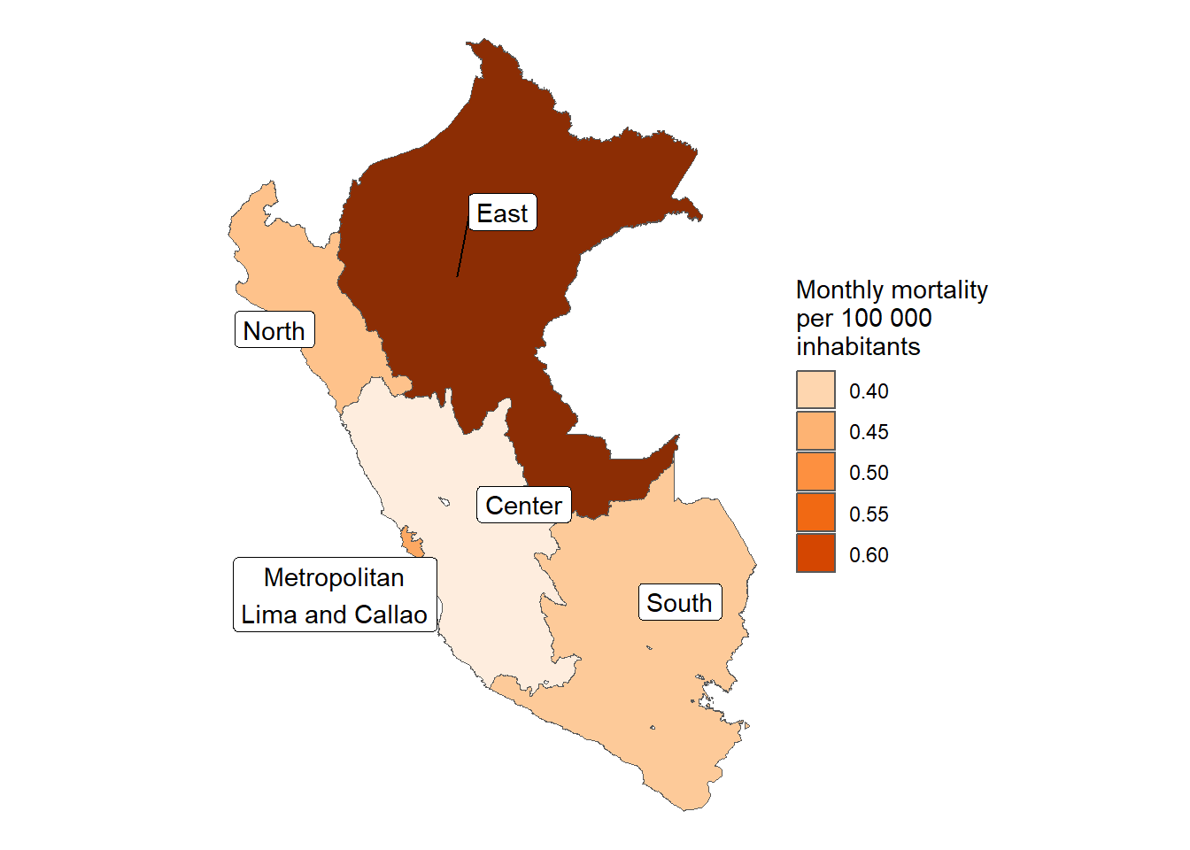
downloadthis::download_file(
  path = "02_output/tables/mortalidad_departamento_edad.xlsx",
  button_label = "Descargar tabla en Excel",
  button_type = "success",
  has_icon = TRUE,
  icon = "fa fa-save"
)

In [189]:

downloadthis::download_file(
  path = "02_output/tables/mortalidad_departamento_edad.docx",
  button_label = "Descargar tabla en Word",
  button_type = "primary",
  has_icon = TRUE,
  icon = "fa fa-save"
)

Macrorregiones - Letalidad

In [190]:

letalidad_macro_100k_sf <- peru_macro_sf %>%
  left_join(
    results_letalidad_overall$macrorregion$index
  )

Joining with `by = join_by(macrorregion)`

In [191]:

let_macro_map <- letalidad_macro_100k_sf %>%
  mutate(
    macrorregion = str_wrap(macrorregion, width = 15)
  ) %>% 
  ggplot() +
  geom_sf(aes(fill = rate)) +
  ggsflabel::geom_sf_label_repel(aes(label = macrorregion),
                                 force = 100,
                                 seed = 2024) +
  guides(
    fill = guide_legend(
      str_wrap("Lethality per 100 cases", 
               20)
    )
  ) +
  scale_fill_distiller(palette = "YlOrBr",
                       direction = 1) + 
  theme_void()

let_macro_map

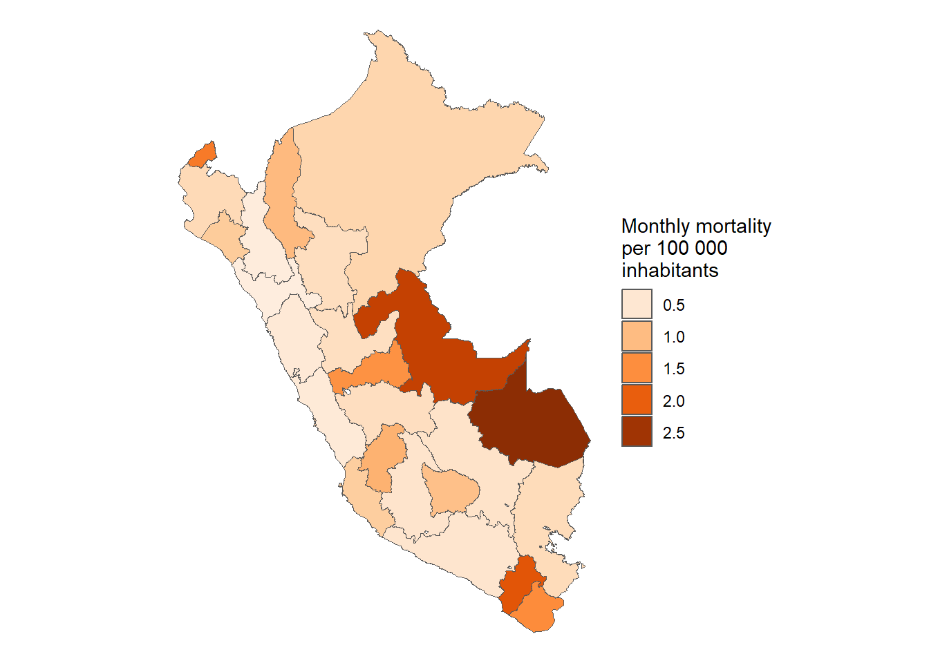
Warning in st_point_on_surface.sfc(data$geometry): st_point_on_surface may not
give correct results for longitude/latitude data

Figura 26: Letalidad COVID-19 por 100K habitantes de acuerdo a la macrorregión (14-03-2020 a 13-06-2023)

Distrital y pobreza

In [192]:

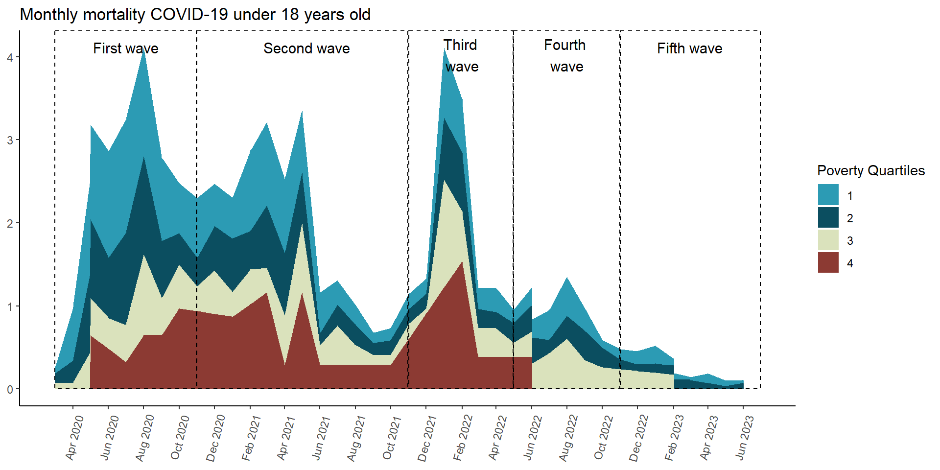
mort_pobr_area_plot <- 
  results_per_month_mortalidad$cuartil_pobreza$index %>% 
  drop_na() %>% 
  mutate(
    time = make_date(anio, mes, "1")
  ) %>% 
  ggplot(
    aes(x = time,
        y = rate,
        fill = cuartil_pobreza)
  ) +
  geom_area(position = 'stack') +
  # innovar::scale_fill_innova("jama") +
  scale_fill_manual(
    values = c("#2C9BB4", "#0B4E60", "#DAE2BC", "#8C3A33")
  ) +
  scale_x_date(
    limits = c(ymd("2020-03-01"), ymd("2023-07-01")),
    breaks = seq(from = ceiling_date(ymd("2020-03-01"), "month"),
                 to = floor_date(ymd("2023-07-01"), "month"),
                 by = "2 months"), 
    # date_breaks = "2 month",
    date_labels = "%b %Y"
  ) +
  labs(
    y = NULL,
    x = NULL,
    title = "Monthly mortality COVID-19 under 18 years old",
    fill = "Poverty Quartiles"
  ) + 
  annotate(
    geom = "rect",
    xmin = as.Date("2020-03-01"), 
    xmax = as.Date("2020-10-31"), 
    ymin = 0, # El rectángulo se extiende hasta la parte inferior del gráfico
    ymax = Inf, # El rectángulo se extiende hasta la parte superior del gráfico
    color = "black", # Color de la línea
    fill = NA, # Sin relleno
    linetype = "dashed", # Tipo de línea discontinua
    linewidth = 0.5 # Grosor de la línea
  ) + 
  annotate(
    geom = "text", 
    x = as.Date("2020-07-01"), # Punto medio aproximado de la Ola 2
    y = Inf, # Posición vertical del texto
    label = "First wave", 
    color = "black",
    size = 4, # Tamaño del texto
    vjust = 2 # Ajuste vertical para colocar el texto encima del rectángulo
  ) +
  annotate(
    geom = "rect",
    xmin = as.Date("2020-11-01"), 
    xmax = as.Date("2021-10-31"), 
    ymin = 0, # El rectángulo se extiende hasta la parte inferior del gráfico
    ymax = Inf, # El rectángulo se extiende hasta la parte superior del gráfico
    color = "black", # Color de la línea
    fill = NA, # Sin relleno
    linetype = "dashed", # Tipo de línea discontinua
    linewidth = 0.5 # Grosor de la línea
  ) + 
  annotate(
    geom = "text", 
    x = as.Date("2021-05-10"), # Punto medio aproximado de la Ola 2
    y = Inf, # Posición vertical del texto
    label = "Second wave", 
    color = "black",
    size = 4, # Tamaño del texto
    vjust = 2 # Ajuste vertical para colocar el texto encima del rectángulo
  ) + 
  annotate(
    geom = "rect",
    xmin = as.Date("2021-11-01"), 
    xmax = as.Date("2022-04-30"), 
    ymin = 0, # El rectángulo se extiende hasta la parte inferior del gráfico
    ymax = Inf, # El rectángulo se extiende hasta la parte superior del gráfico
    color = "black", # Color de la línea
    fill = NA, # Sin relleno
    linetype = "dashed", # Tipo de línea discontinua
    linewidth = 0.5 # Grosor de la línea
  ) + 
  annotate(
    geom = "text", 
    x = as.Date("2022-02-01"), # Punto medio aproximado de la Ola 2
    y = Inf, # Posición vertical del texto
    label = "Third \nwave", 
    color = "black",
    size = 4, # Tamaño del texto
    vjust = 1.25 # Ajuste vertical para colocar el texto encima del rectángulo
  ) + 
  annotate(
    geom = "rect",
    xmin = as.Date("2022-05-01"), 
    xmax = as.Date("2022-10-31"), 
    ymin = 0, # El rectángulo se extiende hasta la parte inferior del gráfico
    ymax = Inf, # El rectángulo se extiende hasta la parte superior del gráfico
    color = "black", # Color de la línea
    fill = NA, # Sin relleno
    linetype = "dashed", # Tipo de línea discontinua
    linewidth = 0.5 # Grosor de la línea
  ) + 
  annotate(
    geom = "text", 
    x = as.Date("2022-08-01"), # Punto medio aproximado de la Ola 2
    y = Inf, # Posición vertical del texto
    label = "Fourth \nwave", 
    color = "black",
    size = 4, # Tamaño del texto
    vjust = 1.25 # Ajuste vertical para colocar el texto encima del rectángulo
  ) +
  annotate(
    geom = "rect",
    xmin = as.Date("2022-11-01"), 
    xmax = as.Date("2023-07-01"), 
    ymin = 0, # El rectángulo se extiende hasta la parte inferior del gráfico
    ymax = Inf, # El rectángulo se extiende hasta la parte superior del gráfico
    color = "black", # Color de la línea
    fill = NA, # Sin relleno
    linetype = "dashed", # Tipo de línea discontinua
    linewidth = 0.5 # Grosor de la línea
  ) + 
  annotate(
    geom = "text", 
    x = as.Date("2023-03-01"),
    y = Inf, # Posición vertical del texto
    label = "Fifth wave", 
    color = "black",
    size = 4, # Tamaño del texto
    vjust = 2 # Ajuste vertical para colocar el texto encima del rectángulo
  ) +
  theme_classic() +
  theme(
    axis.text.x = element_text(
      angle = 75,
      vjust = 0.5
    ),
    axis.ticks.x = element_line()
  ) 

mort_pobr_area_plot

Figura 27: Mortalidad COVID-19 de acuerdo al cuartil de pobreza(14-03-2020 a 13-06-2023)

In [193]:

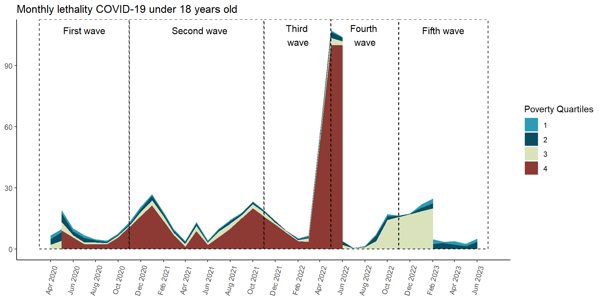
letal_pobr_area_plot <- 
  results_per_month_letalidad$cuartil_pobreza$index %>% 
  drop_na() %>% 
  mutate(
    time = make_date(anio, mes, "1")
  ) %>% 
  filter(
    time > ymd("2020-03-01")
  ) |> 
  ggplot(
    aes(x = time,
        y = rate,
        fill = cuartil_pobreza)
  ) +
  geom_area(position = 'stack') +
  # innovar::scale_fill_innova("jama") +
  scale_fill_manual(
    values = c("#2C9BB4", "#0B4E60", "#DAE2BC", "#8C3A33")
  ) +
  scale_x_date(
    limits = c(ymd("2020-03-01"), ymd("2023-07-01")),
    breaks = seq(from = ceiling_date(ymd("2020-03-01"), "month"),
                 to = floor_date(ymd("2023-07-01"), "month"),
                 by = "2 months"), 
    # date_breaks = "2 month",
    date_labels = "%b %Y"
  ) +
  labs(
    y = NULL,
    x = NULL,
    title = "Monthly lethality COVID-19 under 18 years old",
    fill = "Poverty Quartiles"
  ) + 
  annotate(
    geom = "rect",
    xmin = as.Date("2020-03-01"), 
    xmax = as.Date("2020-10-31"), 
    ymin = 0, # El rectángulo se extiende hasta la parte inferior del gráfico
    ymax = Inf, # El rectángulo se extiende hasta la parte superior del gráfico
    color = "black", # Color de la línea
    fill = NA, # Sin relleno
    linetype = "dashed", # Tipo de línea discontinua
    linewidth = 0.5 # Grosor de la línea
  ) + 
  annotate(
    geom = "text", 
    x = as.Date("2020-07-01"), # Punto medio aproximado de la Ola 2
    y = Inf, # Posición vertical del texto
    label = "First wave", 
    color = "black",
    size = 4, # Tamaño del texto
    vjust = 2 # Ajuste vertical para colocar el texto encima del rectángulo
  ) +
  annotate(
    geom = "rect",
    xmin = as.Date("2020-11-01"), 
    xmax = as.Date("2021-10-31"), 
    ymin = 0, # El rectángulo se extiende hasta la parte inferior del gráfico
    ymax = Inf, # El rectángulo se extiende hasta la parte superior del gráfico
    color = "black", # Color de la línea
    fill = NA, # Sin relleno
    linetype = "dashed", # Tipo de línea discontinua
    linewidth = 0.5 # Grosor de la línea
  ) + 
  annotate(
    geom = "text", 
    x = as.Date("2021-05-10"), # Punto medio aproximado de la Ola 2
    y = Inf, # Posición vertical del texto
    label = "Second wave", 
    color = "black",
    size = 4, # Tamaño del texto
    vjust = 2 # Ajuste vertical para colocar el texto encima del rectángulo
  ) + 
  annotate(
    geom = "rect",
    xmin = as.Date("2021-11-01"), 
    xmax = as.Date("2022-04-30"), 
    ymin = 0, # El rectángulo se extiende hasta la parte inferior del gráfico
    ymax = Inf, # El rectángulo se extiende hasta la parte superior del gráfico
    color = "black", # Color de la línea
    fill = NA, # Sin relleno
    linetype = "dashed", # Tipo de línea discontinua
    linewidth = 0.5 # Grosor de la línea
  ) + 
  annotate(
    geom = "text", 
    x = as.Date("2022-02-01"), # Punto medio aproximado de la Ola 2
    y = Inf, # Posición vertical del texto
    label = "Third \nwave", 
    color = "black",
    size = 4, # Tamaño del texto
    vjust = 1.25 # Ajuste vertical para colocar el texto encima del rectángulo
  ) + 
  annotate(
    geom = "rect",
    xmin = as.Date("2022-05-01"), 
    xmax = as.Date("2022-10-31"), 
    ymin = 0, # El rectángulo se extiende hasta la parte inferior del gráfico
    ymax = Inf, # El rectángulo se extiende hasta la parte superior del gráfico
    color = "black", # Color de la línea
    fill = NA, # Sin relleno
    linetype = "dashed", # Tipo de línea discontinua
    linewidth = 0.5 # Grosor de la línea
  ) + 
  annotate(
    geom = "text", 
    x = as.Date("2022-08-01"), # Punto medio aproximado de la Ola 2
    y = Inf, # Posición vertical del texto
    label = "Fourth \nwave", 
    color = "black",
    size = 4, # Tamaño del texto
    vjust = 1.25 # Ajuste vertical para colocar el texto encima del rectángulo
  ) +
  annotate(
    geom = "rect",
    xmin = as.Date("2022-11-01"), 
    xmax = as.Date("2023-07-01"), 
    ymin = 0, # El rectángulo se extiende hasta la parte inferior del gráfico
    ymax = Inf, # El rectángulo se extiende hasta la parte superior del gráfico
    color = "black", # Color de la línea
    fill = NA, # Sin relleno
    linetype = "dashed", # Tipo de línea discontinua
    linewidth = 0.5 # Grosor de la línea
  ) + 
  annotate(
    geom = "text", 
    x = as.Date("2023-03-01"),
    y = Inf, # Posición vertical del texto
    label = "Fifth wave", 
    color = "black",
    size = 4, # Tamaño del texto
    vjust = 2 # Ajuste vertical para colocar el texto encima del rectángulo
  ) +
  theme_classic() +
  theme(
    axis.text.x = element_text(
      angle = 75,
      vjust = 0.5
    ),
    axis.ticks.x = element_line()
  ) 

letal_pobr_area_plot

Letalidad COVID-19 de acuerdo al cuartil de pobreza(14-03-2020 a 13-06-2023)

Distrito Lima

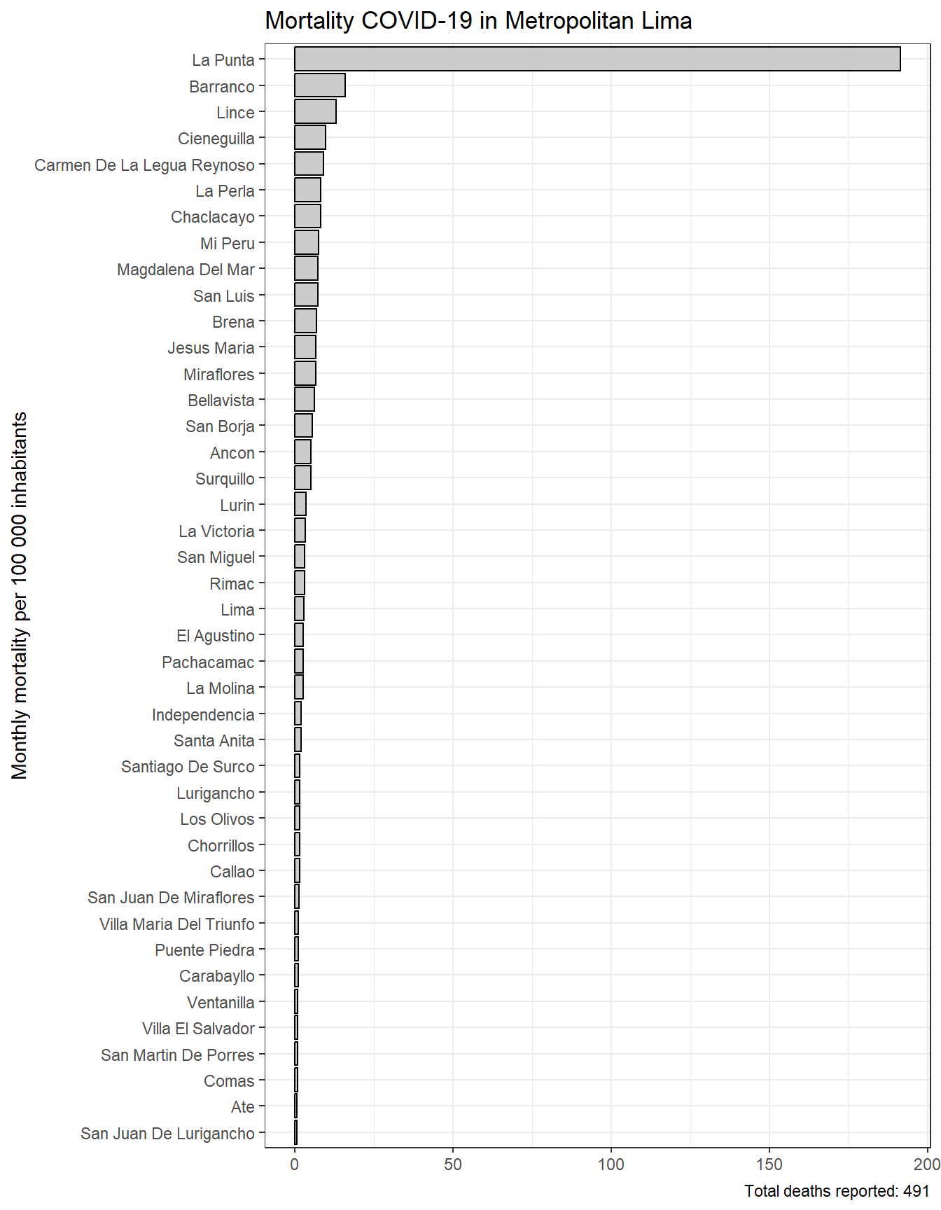
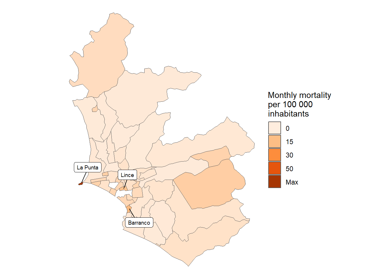
In [194]:

total_mort_distr_lim_callao <- results_mortalidad$distrito$index_pre %>% 
  filter(provincia %in% c("LIMA", "CALLAO")) %>% 
  pull(count) %>% 
  sum()

results_mortalidad$distrito$index %>% 
  filter(provincia %in% c("LIMA", "CALLAO")) %>% 
  mutate(
    distrito = str_to_title(distrito), 
    distrito = fct_reorder(distrito, rate)
  ) %>% 
  ggplot(aes(y = distrito, x = rate)) +
  geom_bar(stat = "identity",
           color = "black",
           fill = "grey80") +
  theme_bw() +
  labs(title = "Mortality COVID-19 in Metropolitan Lima", 
       x = NULL, 
       y = "Mean monthly COVID-19 mortality per 100 000 inhabitants",
       caption = paste0("Total deaths reported: ", 
                        scales::number(total_mort_distr_lim_callao))) +
  innovar::scale_fill_innova("blue_fall") +
  theme(
    legend.position = "bottom"
  )

Figura 28: Mortalidad COVID-19 de acuerdo a los distritos de lima metropolitana (14-03-2020 a 13-06-2023)

In [195]:

mort_lima_distr_1k_sf <- Peru %>% 
  inner_join(
    results_mortalidad$distrito$index %>% 
      filter(provincia %in% c("LIMA", "CALLAO"))
  )

Joining with `by = join_by(ubigeo)`

In [196]:

mort_lima_distr_1k_sf %>%
  mutate(
    label = case_when(
      rate > 10 ~ str_to_title(distrito)
    )
  ) %>%
  ggplot() +
  geom_sf(aes(fill = rate)) +
  guides(
    fill = guide_legend(
      str_wrap("Mean monthly COVID-19 mortality per 100 000 inhabitants", 
               20)
    )
  ) +
  ggsflabel::geom_sf_label_repel(aes(label = label),
                                 force = 10,
                                 size = 2.45,
                                 box.padding = 0.75,
                                 seed = 2024) +
  # scale_fill_distiller(palette = "YlOrBr",
  #                      direction = 1) + 
  scale_fill_gradientn(
    colors = scales::pal_brewer("seq", "Oranges", 1)(5),
    values = scales::rescale(c(0, 15, 30, 50, max(mort_lima_distr_1k_sf$rate, na.rm = TRUE))),
    breaks = c(0, 15, 30, 50, max(mort_lima_distr_1k_sf$rate, na.rm = TRUE)),
    labels = c("0", "15", "30", "50", "Max"),
    limits = c(0,
               max(mort_lima_distr_1k_sf$rate, na.rm = TRUE))
  ) +
  theme_void()

Warning in st_point_on_surface.sfc(data$geometry): st_point_on_surface may not
give correct results for longitude/latitude data

Warning: Removed 39 rows containing missing values or values outside the scale range
(`geom_label_repel()`).

Figura 29: Mortalidad COVID-19 de acuerdo a los distritos de lima metropolitana (14-03-2020 a 13-06-2023)

In [197]:

In [198]:

tbl_summ_mort_lima_distr_pre <- results_mortalidad$distrito$index %>% 
      filter(provincia %in% c("LIMA", "CALLAO")) %>% 
  mutate(
    across(
      departamento:distrito,
      str_to_title
    ),
    rate = formattable::digits(rate, 3)
  ) %>% 
  select(-departamento)

tbl_summ_mort_lima_distr <- tbl_summ_mort_lima_distr_pre %>% 
  rename_with(
    .fn = ~ paste0("**", str_to_title(.x), "**")
  ) %>% 
  gt::gt() %>% 
  gt::cols_label(
    .fn = gt::md,
    .process_units = TRUE
  )

tbl_summ_mort_lima_distr

Tabla 25: Mortalidad COVID-19 de acuerdo a los distritos de lima metropolitana (14-03-2020 a 13-06-2023)

Ubigeo	Provincia	Distrito	Rate
070101	Callao	Callao	1.491
070102	Callao	Bellavista	6.214
070103	Callao	Carmen De La Legua Reynoso	9.212
070104	Callao	La Perla	8.304
070105	Callao	La Punta	191.205
070106	Callao	Ventanilla	1.009
070107	Callao	Mi Peru	7.510
150101	Lima	Lima	2.874
150102	Lima	Ancon	5.237
150103	Lima	Ate	0.808
150104	Lima	Barranco	16.049
150105	Lima	Brena	6.917
150106	Lima	Carabayllo	1.115
150107	Lima	Chaclacayo	8.199
150108	Lima	Chorrillos	1.506
150109	Lima	Cieneguilla	9.741
150110	Lima	Comas	0.828
150111	Lima	El Agustino	2.655
150112	Lima	Independencia	2.099
150113	Lima	Jesus Maria	6.746
150114	Lima	La Molina	2.613
150115	Lima	La Victoria	3.441
150116	Lima	Lince	13.056
150117	Lima	Los Olivos	1.515
150118	Lima	Lurigancho	1.646
150119	Lima	Lurin	3.601
150120	Lima	Magdalena Del Mar	7.306
150122	Lima	Miraflores	6.576
150123	Lima	Pachacamac	2.613
150125	Lima	Puente Piedra	1.150
150128	Lima	Rimac	3.141
150130	Lima	San Borja	5.662
150132	Lima	San Juan De Lurigancho	0.751
150133	Lima	San Juan De Miraflores	1.427
150134	Lima	San Luis	7.285
150135	Lima	San Martin De Porres	0.871
150136	Lima	San Miguel	3.206
150137	Lima	Santa Anita	2.004
150140	Lima	Santiago De Surco	1.665
150141	Lima	Surquillo	5.151
150142	Lima	Villa El Salvador	0.997
150143	Lima	Villa Maria Del Triunfo	1.195

In [199]:

tbl_summ_mort_lima_distr_pre %>% 
  rename_with(
    .fn = str_to_title
  ) %>% 
  huxtable::as_hux() %>% 
  huxtable::set_bold(1, 1:4) %>% 
  huxtable::quick_xlsx(file = "02_output/tables/mortalidad_lima_distrito.xlsx",
                       open = FALSE)

tbl_summ_mort_lima_distr %>%
  gt::gtsave("02_output/tables/mortalidad_lima_distrito.docx")

In [200]:

downloadthis::download_file(
  path = "02_output/tables/mortalidad_lima_distrito.xlsx",
  button_label = "Descargar tabla en Excel",
  button_type = "success",
  has_icon = TRUE,
  icon = "fa fa-save"
)

In [201]:

downloadthis::download_file(
  path = "02_output/tables/mortalidad_lima_distrito.docx",
  button_label = "Descargar tabla en Word",
  button_type = "primary",
  has_icon = TRUE,
  icon = "fa fa-save"
)

Incidencia mensual del COVID-19

In [202]:

incidencia_positivos <- positivos_0723 %>% 
  mutate(
    #fecha_resultado_floor = floor_date(fecha_resultado, unit = "month"),
    mes = month(fecha_resultado_floor)
  )

In [203]:

n_incidencia_positivos <- incidencia_positivos %>% 
  count() %>% 
  pull(n)

n_wo_id <- incidencia_positivos %>% 
  filter(is.na(id_persona)) %>% 
  count() %>% 
  pull(n)

Los datos utilizados para incidencia positivos tienen datos hasta julio de 2023. Se tiene registro de 315 046 casos positivos menores de 18 años. Para poder analizar la incidencia necesitamos saber que si un caso positivos es nuevo o es una reinfección que no se puede considerar aún como caso nuevo. Se tendrá como criterio 3 meses de espacio entre infecciones. Lamentablemente, incluso en estos datos, hay 12 495 registros sin id_persona.

Criterios para casos positivos y de reinfección:

Hasta 1 mes (30 días), se considera una misma infección.
Espacio de 3 meses a más (90 días), se considera una nueva infección (reinfección)
Reportar cantidad de casos que se encuentren entre 1 mes y menos de 3 meses (entre día 31 y 89), con su respectivo método.

In [204]:

incidencia_positivos %>% 
  count(caso_intermedio)

# Source:   SQL [?? x 2]
# Database: DuckDB v1.2.0 [brian@Windows 10 x64:R 4.4.2/D:\Github\covid-analisis-ninos\01_data\raw\covid.duckdb]
  caso_intermedio      n
  <lgl>            <dbl>
1 FALSE           302236
2 TRUE               245
3 NA               12565

In [205]:

# incidencia_positivos %>% 
#   filter(anio == 2020,
#          !is.na(id_persona)) %>% 
#   group_by(fecha_resultado_floor) %>%
#   summarise(
#     casos_sin_reinfecciones = n_distinct(id_persona),
#     casos_con_reinfeccioens = n()
#   ) %>% 
#   ungroup() %>% 
#   arrange(fecha_resultado_floor) %>% 
#   collect()
# 
# incidencia_positivos %>% 
#   filter(anio == 2020, !is.na(id_persona)) %>% 
#   group_by(fecha_resultado_floor) %>%
#   add_count(id_persona) %>% 
#   filter(n > 1) %>% 
#   select(departamento:fecha_resultado, id_persona)

# incidencia_positivos %>% 
#   filter(anio == 2020) %>% 
#   count(fecha_resultado_floor) %>%
#   ungroup() %>% 
#   arrange(fecha_resultado_floor) %>% 
#   collect()
#   
#   count(
#     across(c(fecha_resultado_floor, departamento:distrito, grupo_edad, sexo))
#   )

Tasa de hospitalización

In [206]:

hospitalizados <- hosp_final %>%
  filter(edad < 18,
         fecha_ingreso_hosp <= max_positivos_0723) %>% 
  mutate(
    mes = month(fecha_ingreso_hosp),
    overall = "overall"
  ) 

range_hospi <- hospitalizados %>% 
  summarise(
    min = min(fecha_ingreso_hosp),
    max = max(fecha_ingreso_hosp)
  ) %>% 
  collect() %>% 
  mutate(
    min = format(min, "%d-%m-%Y"),
    max = format(max, "%d-%m-%Y"),
    fecha = paste0("(", min, " a ", max, ")")
  )

Vista general

Cálculo de Tasa de hospitalización

In [207]:

levels <- list(
  c("overall"),
  c("grupo_edad"),
  c("sexo"),
  c("ola_covid"),
  c("ola_covid", "grupo_edad"),
  c("ola_covid", "sexo"),
  c("ola_covid", "region"),
  c("ola_covid", "macrorregion"),
  c("departamento"),
  c("departamento", "sexo"),
  c("departamento", "grupo_edad"),
  c("departamento", "sexo", "grupo_edad"),
  c("departamento", "ola_covid"),
  c("distrito"),
  c("distrito", "sexo"),
  c("distrito", "grupo_edad"),
  c("distrito", "cuartil_pobreza"),
  c("grupo_edad", "cuartil_pobreza"),
  c("sexo", "cuartil_pobreza"),
  c("ola_covid", "cuartil_pobreza"),
  c("ola_covid", "cuartil_nbi"),
  c("cuartil_pobreza"),
  c("cuartil_nbi"),
  c("region"),
  c("macrorregion")
)

# Calcular la tasa de hospitalizaciones
results_hospi <- index_calculator(
  data = hospitalizados, 
  denom = positivos_0723 %>% 
    mutate(cantidad = 1), 
  levels = levels, 
  type = "overall",
  std = 100
)

results_per_month_hospi <- index_calculator(
  data = hospitalizados, 
  denom = positivos_0723 %>% 
    mutate(cantidad = 1), 
  levels = levels, 
  type = "per_month",
  std = 100
)

In [208]:

hospi_total_df <- hospitalizados %>% 
  select(edad, overall, grupo_edad, sexo, ola_covid, region, 
         macrorregion, cuartil_pobreza, cuartil_nbi) %>% 
  collect()

labelled::var_label(hospi_total_df) <- list(
  overall = "Overall",
  grupo_edad = "Age Group",
  sexo = "Sex",
  ola_covid = "COVID-19 wave",
  region = "Natural Regions",
  macrorregion = "Macroregions",
  cuartil_pobreza = "Poverty level",
  cuartil_nbi = "Unsatisfied basic needs level"
)

In [209]:

tbl_summ_hospi_g <- hospi_total_df %>% 
  select(overall, grupo_edad, sexo, ola_covid, region, 
         macrorregion, cuartil_pobreza, cuartil_nbi) %>% 
  gtsummary::tbl_summary(
    type = list(
      overall ~ "dichotomous"
    ),
    value = list(overall = "overall"),
    missing_text = "No data"
  ) %>% 
  gtsummary::modify_header(label = "**Variables**") %>%
  gtsummary::bold_labels()

tbl_summ_hospi_c2 <- results_hospi$overall$index %>% 
  mutate(label = "Overall") %>% 
  rename(variable = overall) %>% 
  bind_rows(
    results_hospi$grupo_edad$index %>% 
      mutate(variable = "grupo_edad") %>% 
      rename(label = grupo_edad),
    results_hospi$sexo$index %>% 
      mutate(variable = "sexo") %>% 
      rename(label = sexo),
    results_hospi$ola_covid$index %>% 
      mutate(variable = "ola_covid") %>% 
      rename(label = ola_covid),
    results_hospi$region$index %>% 
      mutate(variable = "region") %>% 
      rename(label = region),
    results_hospi$macrorregion$index %>% 
      mutate(variable = "macrorregion") %>% 
      rename(label = macrorregion),
    results_hospi$cuartil_pobreza$index %>% 
      mutate(variable = "cuartil_pobreza") %>% 
      rename(label = cuartil_pobreza),
    results_hospi$cuartil_nbi$index %>% 
      mutate(variable = "cuartil_nbi") %>% 
      rename(label = cuartil_nbi)
  ) %>% 
  drop_na() %>% 
  mutate(
    rate = formattable::digits(rate, 3)
  )

tbl_summ_hospi_final <- tbl_summ_hospi_g %>%
  gtsummary::modify_table_body(
    ~ .x %>% 
      left_join(tbl_summ_hospi_c2) %>% 
      mutate(
        label = case_when(
          variable %in% c("cuartil_pobreza", "cuartil_nbi") &
            label == "1" ~ "1 (0-19.9%)",
          variable %in% c("cuartil_pobreza", "cuartil_nbi") & 
            label == "2" ~ "2 (20-39.9%)",
          variable %in% c("cuartil_pobreza", "cuartil_nbi") & 
            label == "3" ~ "3 (40-59.9%)",
          variable %in% c("cuartil_pobreza", "cuartil_nbi") &
            label == "4" ~ "4 (60-100%)",
          .default = label
        )
      )
  ) %>% 
  gtsummary::modify_header(
    rate ~ "**Hospital admission rate per 100 cases**"
  ) %>%
  gtsummary::modify_fmt_fun(
    rate ~ scales::number_format(accuracy = 0.001)
  )

Joining with `by = join_by(variable, label)`

In [210]:

tbl_summ_hospi_final

Tabla 26: Descriptivos de Hospitalizados menores de 18 años (24-03-2020 a 16-06-2023)

Variables	N = 6,936¹	Hospital admission rate per 100 cases
Overall	6,936 (100%)	2.202
Age Group
Under 1 year	0 (0%)
1 - 5 years	2,350 (34%)	5.157
6 - 11 years	2,637 (38%)	2.877
12 - 17 years	1,949 (28%)	1.208
Sex
Female	3,097 (45%)	1.941
Male	3,839 (55%)	2.469
COVID-19 wave
1 (Mar – Oct 2020)	1,217 (18%)	2.032
2 (Nov 2020 – Oct 2021)	2,326 (34%)	3.210
3 (Nov 2021 – Apr 2022)	2,018 (29%)	1.899
4 (May 2022 – Oct 2022)	1,075 (15%)	1.848
5 (Nov 2022 – Jun 2023)	300 (4.3%)	1.654
Natural Regions
Coast	5,368 (77%)	2.289
Highlands	917 (13%)	1.700
Jungle	651 (9.4%)	2.445
Macroregions
Center	1,053 (15%)	1.462
East	613 (8.8%)	2.510
Metropolitan Lima and Callao	4,202 (61%)	3.550
North	633 (9.1%)	1.252
South	435 (6.3%)	0.876
Poverty level
1 (0-19.9%)	4,323 (62%)	1.852
2 (20-39.9%)	2,217 (32%)	4.458
3 (40-59.9%)	342 (4.9%)	2.270
4 (60-100%)	54 (0.8%)	3.659
Unsatisfied basic needs level
1 (0-19.9%)	4,129 (60%)	2.178
2 (20-39.9%)	2,146 (31%)	2.650
3 (40-59.9%)	440 (6.3%)	2.447
4 (60-100%)	221 (3.2%)	1.988
¹ n (%)

In [211]:

tbl_summ_hospi_final %>% 
  gtsummary::as_hux_xlsx("02_output/tables/hospitalizacion_descriptivos.xlsx")

tbl_summ_hospi_final %>%
  gtsummary::as_flex_table() %>%
  flextable::save_as_docx(path = "02_output/tables/hospitalizacion_descriptivos.docx")

In [212]:

downloadthis::download_file(
  path = "02_output/tables/hospitalizacion_descriptivos.xlsx",
  button_label = "Descargar tabla en Excel",
  button_type = "success",
  has_icon = TRUE,
  icon = "fa fa-save"
)

In [213]:

downloadthis::download_file(
  path = "02_output/tables/hospitalizacion_descriptivos.docx",
  button_label = "Descargar tabla en Word",
  button_type = "primary",
  has_icon = TRUE,
  icon = "fa fa-save"
)

In [214]:

hospital_comparisons <- compare_levels_per_month(
  results_per_month = results_per_month_hospi,
  levels = comparing_levels
)

# Extraer las tablas `cld` como tibbles, renombrando y añadiendo una columna "level"
hospital_comparisons_cld_pre <- lapply(names(hospital_comparisons), function(level) {
  cld <- hospital_comparisons[[level]]$cld
  
  if (!is.null(cld)) {
    cld <- cld |> 
      as_tibble() |> 
      rename(group = 1) |>  # Renombra la primera columna a 'group'
      mutate(level = level) |> # Añade una columna 'level' con el nombre de la lista
      relocate(level) 
  }
  
  cld
}) |> 
  bind_rows()

hospital_comparisons_cld_pre <- 
  hospital_comparisons_cld_pre |> 
  mutate(
    across(
      where(is.numeric),
      ~ formattable::digits(.x, 3)
    )
  )

In [215]:

In [216]:

hospital_comparisons_cld <- hospital_comparisons_cld_pre |> 
  rename_with(
    .fn = ~ paste0("**", str_to_title(.x), "**")
  ) %>% 
  gt::gt() %>% 
  gt::cols_label(
    .fn = gt::md,
    .process_units = TRUE
  )

hospital_comparisons_cld

Tabla 27: Comparaciones múltiples de hospitalidad(07-03-2020 a 17-06-2023)

Level	Group	Emmean	Se	Df	Lower.cl	Upper.cl	.Group
grupo_edad	12 - 17 years	2.063	1.470	86.747	-0.859	4.984	a
grupo_edad	6 - 11 years	7.977	1.456	85.302	5.083	10.872	b
grupo_edad	1 - 5 years	12.285	1.456	85.302	9.390	15.179	c
sexo	Female	4.231	0.683	40.574	2.852	5.610	a
sexo	Male	5.036	0.683	40.574	3.657	6.415	b
ola_covid	1 (Mar – Oct 2020)	2.185	1.459	35.000	-0.776	5.146	a
ola_covid	2 (Nov 2020 – Oct 2021)	3.980	1.191	35.000	1.562	6.397	a
ola_covid	5 (Nov 2022 – Jun 2023)	4.597	1.459	35.000	1.636	7.558	a
ola_covid	3 (Nov 2021 – Apr 2022)	6.695	1.684	35.000	3.276	10.114	a
ola_covid	4 (May 2022 – Oct 2022)	7.150	1.684	35.000	3.731	10.569	a
cuartil_pobreza	1	4.162	3.185	115.095	-2.148	10.472	a
cuartil_pobreza	3	5.027	3.471	122.597	-1.845	11.898	a
cuartil_pobreza	2	9.025	3.223	115.880	2.641	15.409	a
cuartil_pobreza	4	21.189	3.861	129.645	13.550	28.827	b
cuartil_nbi	3	3.924	1.420	116.753	1.113	6.736	a
cuartil_nbi	1	5.111	1.360	110.055	2.416	7.806	a
cuartil_nbi	2	5.182	1.360	110.055	2.487	7.877	a
cuartil_nbi	4	7.993	1.453	120.380	5.117	10.870	a
region	Highlands	2.984	1.076	100.027	0.849	5.120	a
region	Coast	5.393	1.064	99.517	3.283	7.503	a
region	Jungle	5.597	1.163	104.145	3.291	7.903	a
macrorregion	North	2.522	1.740	152.325	-0.917	5.960	a
macrorregion	Center	2.794	1.741	151.995	-0.645	6.233	a
macrorregion	South	4.057	1.718	150.773	0.663	7.451	a
macrorregion	East	5.781	1.814	157.606	2.199	9.363	ab
macrorregion	Metropolitan Lima and Callao	10.155	1.655	146.304	6.884	13.425	b

In [217]:

hospital_comparisons_cld_pre %>% 
  rename_with(
    .fn = str_to_title
  ) %>% 
  huxtable::as_hux() %>% 
  huxtable::set_bold(1, 1:8) %>% 
  huxtable::quick_xlsx(file = "02_output/tables/hospital_comparacion_multiple.xlsx",
                       open = FALSE)

hospital_comparisons_cld %>%
  gt::gtsave("02_output/tables/hospital_comparacion_multiple.docx")

In [218]:

downloadthis::download_file(
  path = "02_output/tables/hospital_comparacion_multiple.xlsx",
  button_label = "Descargar tabla en Excel",
  button_type = "success",
  has_icon = TRUE,
  icon = "fa fa-save"
)

In [219]:

downloadthis::download_file(
  path = "02_output/tables/hospital_comparacion_multiple.docx",
  button_label = "Descargar tabla en Word",
  button_type = "primary",
  has_icon = TRUE,
  icon = "fa fa-save"
)

In [220]:

tbl_summ_hospi_olas <- hospi_total_df %>% 
  select(overall, grupo_edad, sexo, ola_covid, region, 
         macrorregion, cuartil_pobreza, cuartil_nbi) %>% 
  gtsummary::tbl_summary(
    by = ola_covid,
    type = list(
      overall ~ "dichotomous"
    ),
    value = list(overall = "overall"),
    missing_text = "No data"
  ) %>% 
  gtsummary::modify_header(label = "**Variables**") %>%
  gtsummary::bold_labels()


ola_covid_hospi_gtsumm <- results_hospi$ola_covid$index %>% 
  rename(stat = ola_covid) %>% 
  mutate(label = "Overall",
         variable = "overall") %>% 
  bind_rows(
    results_hospi$ola_covid_grupo_edad$index %>%
      mutate(variable = "grupo_edad") %>% 
      rename(label = grupo_edad,
             stat = ola_covid),
    results_hospi$ola_covid_sexo$index %>% 
      mutate(variable = "sexo") %>% 
      rename(label = sexo,
             stat = ola_covid),
    results_hospi$ola_covid_region$index %>% 
      mutate(variable = "region") %>% 
      rename(label = region,
             stat = ola_covid),
    results_hospi$ola_covid_macrorregion$index %>% 
      mutate(variable = "macrorregion") %>%
      rename(label = macrorregion,
             stat = ola_covid),
    results_hospi$ola_covid_cuartil_pobreza$index %>% 
      mutate(variable = "cuartil_pobreza") %>% 
      rename(label = cuartil_pobreza,
             stat = ola_covid),
    results_hospi$ola_covid_cuartil_nbi$index %>% 
      mutate(variable = "cuartil_nbi") %>% 
      rename(label = cuartil_nbi,
             stat = ola_covid)
  ) %>% 
  mutate(
    rate = formattable::digits(rate, 3),
    stat = as.character(stat),
    stat = case_match(
      stat,
      "1 (Mar – Oct 2020)" ~ "stat_1",
      "2 (Nov 2020 – Oct 2021)" ~ "stat_2",
      "3 (Nov 2021 – Apr 2022)" ~ "stat_3",
      "4 (May 2022 – Oct 2022)" ~ "stat_4",
      "5 (Nov 2022 – Jun 2023)" ~ "stat_5"
    )
  ) 


tbl_summ_hospi_olas$table_body <- tbl_summ_hospi_olas$table_body %>%
  mutate(
    across(
      gtsummary::all_stat_cols(stat_0 = FALSE),
      ~ str_remove_all(., "\\s*\\(.*?\\)\\s*")
    )
  ) %>% 
  pivot_longer(
    cols = stat_1:stat_5,
    names_to = "stat",
    values_to = "freq"
  ) %>% 
  left_join(
    ola_covid_hospi_gtsumm
  ) %>% 
  mutate(
    value = str_c(freq, ifelse(is.na(rate), "", str_c(" (", rate, ")")))
  ) %>% 
  select(-c(freq, rate)) %>% 
  pivot_wider(
    names_from = stat,
    values_from = value
  )

Joining with `by = join_by(variable, label, stat)`

In [221]:

tbl_summ_hospi_olas <- tbl_summ_hospi_olas %>% 
  gtsummary::modify_footnote(
    gtsummary::all_stat_cols() ~ "n (HAR per 100 cases)"
  )

tbl_summ_hospi_olas

Tabla 28: Descriptivos de hospitalizados menores de 18 años por olas (24-03-2020 a 16-06-2023)

Variables	1 (Mar – Oct 2020) N = 1,217¹	2 (Nov 2020 – Oct 2021) N = 2,326¹	3 (Nov 2021 – Apr 2022) N = 2,018¹	4 (May 2022 – Oct 2022) N = 1,075¹	5 (Nov 2022 – Jun 2023) N = 300¹
Overall	1,217 (2.032)	2,326 (3.210)	2,018 (1.899)	1,075 (1.848)	300 (1.654)
Age Group
Under 1 year	0	0	0	0	0
1 - 5 years	246 (1.945)	654 (7.166)	846 (5.349)	498 (8.037)	106 (5.952)
6 - 11 years	522 (3.190)	926 (5.295)	673 (1.781)	372 (2.245)	144 (4.199)
12 - 17 years	449 (1.747)	746 (1.728)	499 (1.036)	205 (0.621)	50 (0.448)
Sex
Female	537 (1.732)	1,007 (2.760)	898 (1.686)	499 (1.685)	156 (1.695)
Male	680 (2.354)	1,319 (3.665)	1,120 (2.111)	576 (2.017)	144 (1.611)
Natural Regions
Coast	742 (1.890)	1,727 (3.400)	1,669 (1.964)	958 (2.150)	272 (1.833)
Highlands	190 (2.057)	340 (2.299)	283 (1.664)	83 (0.799)	21 (0.833)
Jungle	285 (2.501)	259 (3.760)	66 (1.529)	34 (1.048)	7 (0.896)
Macroregions
Center	191 (1.460)	315 (1.857)	345 (1.423)	185 (1.397)	17 (0.378)
East	270 (2.587)	246 (3.807)	65 (1.634)	25 (0.878)	7 (1.003)
Metropolitan Lima and Callao	481 (2.344)	1,404 (5.263)	1,311 (3.226)	761 (3.324)	245 (3.220)
North	192 (2.088)	220 (1.885)	164 (0.867)	44 (0.509)	13 (0.613)
South	83 (1.247)	141 (1.318)	133 (0.718)	60 (0.568)	18 (0.560)
Poverty level
1	861 (2.057)	1,481 (2.908)	1,144 (1.407)	597 (1.324)	240 (1.702)
2	285 (2.509)	684 (5.128)	758 (5.080)	440 (5.586)	50 (2.244)
3	59 (1.375)	135 (3.234)	105 (2.575)	34 (1.603)	9 (2.261)
4	12 (3.750)	26 (6.103)	11 (3.056)	4 (1.361)	1 (1.316)
Unsatisfied basic needs level
1	554 (1.837)	1,397 (3.396)	1,236 (1.820)	708 (1.852)	234 (1.937)
2	434 (2.397)	669 (3.419)	671 (2.614)	324 (2.375)	48 (1.208)
3	173 (3.559)	151 (2.898)	77 (1.577)	27 (1.084)	12 (2.251)
4	56 (1.188)	109 (3.689)	34 (1.541)	16 (1.562)	6 (2.791)
¹ n (HAR per 100 cases)

In [222]:

tbl_summ_hospi_olas %>% 
  gtsummary::as_hux_xlsx("02_output/tables/hospitalizados_olas_descriptivos.xlsx")

tbl_summ_hospi_olas %>%
  gtsummary::as_flex_table() %>%
  flextable::save_as_docx(path = "02_output/tables/hospitalizados_olas_descriptivos.docx")

In [223]:

downloadthis::download_file(
  path = "02_output/tables/hospitalizados_olas_descriptivos.xlsx",
  button_label = "Descargar tabla en Excel",
  button_type = "success",
  has_icon = TRUE,
  icon = "fa fa-save"
)

In [224]:

downloadthis::download_file(
  path = "02_output/tables/hospitalizados_olas_descriptivos.docx",
  button_label = "Descargar tabla en Word",
  button_type = "primary",
  has_icon = TRUE,
  icon = "fa fa-save"
)

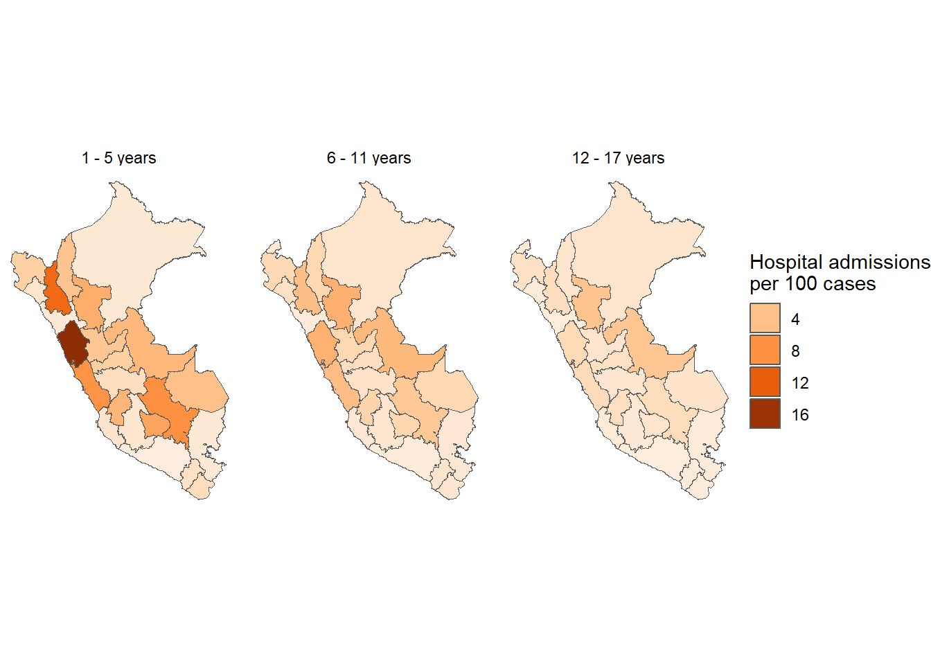
Gráfico de hospitalización (serie de tiempo) - Menores de 18 años

In [225]:

hospi_count_by_age_area <- hospitalizados %>% 
  to_arrow() %>% 
  mutate(
    fecha_round = ceiling_date(fecha_ingreso_hosp, unit = "month")
  ) %>%
  compute() %>% 
  to_duckdb() %>% 
  mutate(
    fecha_round = case_when(
      fecha_round == as.Date("2024-01-01") ~  as.Date("2023-12-31"),
      .default = fecha_round
    )
  ) %>%
  count(grupo_edad, fecha_round) %>% 
  collect()

hospi_age_area_plot <- hospi_count_by_age_area %>% 
  bind_rows(
    tibble(
      grupo_edad = "Under 1 year",
      fecha_round = seq(from = as.Date("2020-04-01"), to = as.Date("2023-07-01"), by = "month"),
      n = 0
    )
  ) %>% 
  mutate(
    grupo_edad = factor(
      grupo_edad,
      levels = c("Under 1 year", "1 - 5 years",
                 "6 - 11 years", "12 - 17 years")
    )
  ) %>% 
  ggplot(
    aes(
      x = fecha_round,
      y = n,
      fill = grupo_edad
    )
  ) +
  geom_area(position = 'stack') +
  # innovar::scale_fill_innova("jama") +
  scale_fill_manual(
    values = c("#2C9BB4", "#0B4E60", "#DAE2BC", "#8C3A33")
  ) +
  scale_x_date(
    limits = c(ymd("2020-03-07"), ymd("2023-07-01")),
    breaks = seq(from = ceiling_date(ymd("2020-03-07"), "month"),
                 to = floor_date(ymd("2023-07-01"), "month"),
                 by = "2 months"), 
    # date_breaks = "2 month",
    date_labels = "%b %Y"
  ) +
  labs(
    y = NULL,
    x = NULL,
    title = "COVID-19 hospital admissions",
    fill = "Age Group"
  ) + 
  annotate(
    geom = "rect",
    xmin = as.Date("2020-04-01"), 
    xmax = as.Date("2020-10-31"), 
    ymin = 0, # El rectángulo se extiende hasta la parte inferior del gráfico
    ymax = Inf, # El rectángulo se extiende hasta la parte superior del gráfico
    color = "black", # Color de la línea
    fill = NA, # Sin relleno
    linetype = "dashed", # Tipo de línea discontinua
    linewidth = 0.5 # Grosor de la línea
  ) + 
  annotate(
    geom = "text", 
    x = as.Date("2020-07-15"), # Punto medio aproximado de la Ola 2
    y = Inf, # Posición vertical del texto
    label = "First wave", 
    color = "black",
    size = 4, # Tamaño del texto
    vjust = 2 # Ajuste vertical para colocar el texto encima del rectángulo
  ) +
  annotate(
    geom = "rect",
    xmin = as.Date("2020-11-01"), 
    xmax = as.Date("2021-10-31"), 
    ymin = 0, # El rectángulo se extiende hasta la parte inferior del gráfico
    ymax = Inf, # El rectángulo se extiende hasta la parte superior del gráfico
    color = "black", # Color de la línea
    fill = NA, # Sin relleno
    linetype = "dashed", # Tipo de línea discontinua
    linewidth = 0.5 # Grosor de la línea
  ) + 
  annotate(
    geom = "text", 
    x = as.Date("2021-05-10"), # Punto medio aproximado de la Ola 2
    y = Inf, # Posición vertical del texto
    label = "Second wave", 
    color = "black",
    size = 4, # Tamaño del texto
    vjust = 2 # Ajuste vertical para colocar el texto encima del rectángulo
  ) + 
  annotate(
    geom = "rect",
    xmin = as.Date("2021-11-01"), 
    xmax = as.Date("2022-04-30"), 
    ymin = 0, # El rectángulo se extiende hasta la parte inferior del gráfico
    ymax = Inf, # El rectángulo se extiende hasta la parte superior del gráfico
    color = "black", # Color de la línea
    fill = NA, # Sin relleno
    linetype = "dashed", # Tipo de línea discontinua
    linewidth = 0.5 # Grosor de la línea
  ) + 
    annotate(
    geom = "text", 
    x = as.Date("2022-02-01"), # Punto medio aproximado de la Ola 2
    y = Inf, # Posición vertical del texto
    label = "Third \nwave", 
    color = "black",
    size = 4, # Tamaño del texto
    vjust = 1.25 # Ajuste vertical para colocar el texto encima del rectángulo
  ) + 
  annotate(
    geom = "rect",
    xmin = as.Date("2022-05-01"), 
    xmax = as.Date("2022-10-31"), 
    ymin = 0, # El rectángulo se extiende hasta la parte inferior del gráfico
    ymax = Inf, # El rectángulo se extiende hasta la parte superior del gráfico
    color = "black", # Color de la línea
    fill = NA, # Sin relleno
    linetype = "dashed", # Tipo de línea discontinua
    linewidth = 0.5 # Grosor de la línea
  ) + 
  annotate(
    geom = "text", 
    x = as.Date("2022-08-01"), # Punto medio aproximado de la Ola 2
    y = Inf, # Posición vertical del texto
    label = "Fourth \nwave", 
    color = "black",
    size = 4, # Tamaño del texto
    vjust = 1.25 # Ajuste vertical para colocar el texto encima del rectángulo
  ) +
  annotate(
    geom = "rect",
    xmin = as.Date("2022-11-01"), 
    xmax = as.Date("2023-07-01"), 
    ymin = 0, # El rectángulo se extiende hasta la parte inferior del gráfico
    ymax = Inf, # El rectángulo se extiende hasta la parte superior del gráfico
    color = "black", # Color de la línea
    fill = NA, # Sin relleno
    linetype = "dashed", # Tipo de línea discontinua
    linewidth = 0.5 # Grosor de la línea
  ) + 
  annotate(
    geom = "text", 
    x = as.Date("2023-03-01"),
    y = Inf, # Posición vertical del texto
    label = "Fifth wave", 
    color = "black",
    size = 4, # Tamaño del texto
    vjust = 2 # Ajuste vertical para colocar el texto encima del rectángulo
  ) +
  theme_classic() +
  theme(
    axis.text.x = element_text(
      angle = 75,
      vjust = 0.5
    ),
    axis.ticks.x = element_line()
  ) 

hospi_age_area_plot

Figura 30: Hospitalización COVID-19 de acuerdo a la edad y ola covid (24-03-2020 a 16-06-2023)

Gráfico Tasa de hospitalización (serie de tiempo)

In [226]:

per_month_hospi_under_1 <- tibble(
  grupo_edad = "Under 1 year",
  time = seq(from = as.Date("2020-03-01"), to = as.Date("2023-07-01"), by = "month"),
  rate = 0
)

hospi_rate_by_age_area <- results_per_month_hospi$grupo_edad$index %>% 
  mutate(
    time = make_date(anio, mes, "1")
  ) %>% 
  bind_rows(
    per_month_hospi_under_1
  ) %>%  
  mutate(
    grupo_edad = factor(
      grupo_edad,
      levels = c("Under 1 year", "1 - 5 years",
                 "6 - 11 years", "12 - 17 years")
    )
  ) %>% 
  ggplot(
    aes(
      x = time,
      y = rate,
      fill = grupo_edad
    )
  ) +
  geom_area(position = 'stack') +
  scale_fill_manual(
    values = c("#2C9BB4", "#0B4E60", "#DAE2BC", "#8C3A33")
  ) +
  scale_x_date(
    limits = c(ymd("2020-03-01"), ymd("2023-07-01")),
    breaks = seq(from = ceiling_date(ymd("2020-03-01"), "month"),
                 to = floor_date(ymd("2023-07-01"), "month"),
                 by = "2 months"), 
    # date_breaks = "2 month",
    date_labels = "%b %Y"
  ) +
  labs(
    y = NULL,
    x = NULL,
    title = "Monthly COVID-19 hospital admission rate per 100 cases",
    fill = "Age Group"
  ) + 
  annotate(
    geom = "rect",
    xmin = as.Date("2020-03-01"), 
    xmax = as.Date("2020-10-31"), 
    ymin = 0, # El rectángulo se extiende hasta la parte inferior del gráfico
    ymax = Inf, # El rectángulo se extiende hasta la parte superior del gráfico
    color = "black", # Color de la línea
    fill = NA, # Sin relleno
    linetype = "dashed", # Tipo de línea discontinua
    linewidth = 0.5 # Grosor de la línea
  ) + 
  annotate(
    geom = "text", 
    x = as.Date("2020-07-01"), # Punto medio aproximado de la Ola 2
    y = Inf, # Posición vertical del texto
    label = "First wave", 
    color = "black",
    size = 4, # Tamaño del texto
    vjust = 2 # Ajuste vertical para colocar el texto encima del rectángulo
  ) +
  annotate(
    geom = "rect",
    xmin = as.Date("2020-11-01"), 
    xmax = as.Date("2021-10-31"), 
    ymin = 0, # El rectángulo se extiende hasta la parte inferior del gráfico
    ymax = Inf, # El rectángulo se extiende hasta la parte superior del gráfico
    color = "black", # Color de la línea
    fill = NA, # Sin relleno
    linetype = "dashed", # Tipo de línea discontinua
    linewidth = 0.5 # Grosor de la línea
  ) + 
  annotate(
    geom = "text", 
    x = as.Date("2021-05-10"), # Punto medio aproximado de la Ola 2
    y = Inf, # Posición vertical del texto
    label = "Second wave", 
    color = "black",
    size = 4, # Tamaño del texto
    vjust = 2 # Ajuste vertical para colocar el texto encima del rectángulo
  ) + 
  annotate(
    geom = "rect",
    xmin = as.Date("2021-11-01"), 
    xmax = as.Date("2022-04-30"), 
    ymin = 0, # El rectángulo se extiende hasta la parte inferior del gráfico
    ymax = Inf, # El rectángulo se extiende hasta la parte superior del gráfico
    color = "black", # Color de la línea
    fill = NA, # Sin relleno
    linetype = "dashed", # Tipo de línea discontinua
    linewidth = 0.5 # Grosor de la línea
  ) + 
    annotate(
    geom = "text", 
    x = as.Date("2022-02-01"), # Punto medio aproximado de la Ola 2
    y = Inf, # Posición vertical del texto
    label = "Third \nwave", 
    color = "black",
    size = 4, # Tamaño del texto
    vjust = 1.25 # Ajuste vertical para colocar el texto encima del rectángulo
  ) + 
  annotate(
    geom = "rect",
    xmin = as.Date("2022-05-01"), 
    xmax = as.Date("2022-10-31"), 
    ymin = 0, # El rectángulo se extiende hasta la parte inferior del gráfico
    ymax = Inf, # El rectángulo se extiende hasta la parte superior del gráfico
    color = "black", # Color de la línea
    fill = NA, # Sin relleno
    linetype = "dashed", # Tipo de línea discontinua
    linewidth = 0.5 # Grosor de la línea
  ) + 
  annotate(
    geom = "text", 
    x = as.Date("2022-08-01"), # Punto medio aproximado de la Ola 2
    y = Inf, # Posición vertical del texto
    label = "Fourth \nwave", 
    color = "black",
    size = 4, # Tamaño del texto
    vjust = 1.25 # Ajuste vertical para colocar el texto encima del rectángulo
  ) +
  annotate(
    geom = "rect",
    xmin = as.Date("2022-11-01"), 
    xmax = as.Date("2023-07-01"), 
    ymin = 0, # El rectángulo se extiende hasta la parte inferior del gráfico
    ymax = Inf, # El rectángulo se extiende hasta la parte superior del gráfico
    color = "black", # Color de la línea
    fill = NA, # Sin relleno
    linetype = "dashed", # Tipo de línea discontinua
    linewidth = 0.5 # Grosor de la línea
  ) + 
  annotate(
    geom = "text", 
    x = as.Date("2023-03-01"),
    y = Inf, # Posición vertical del texto
    label = "Fifth wave", 
    color = "black",
    size = 4, # Tamaño del texto
    vjust = 2 # Ajuste vertical para colocar el texto encima del rectángulo
  ) +
  theme_classic() +
  theme(
    axis.text.x = element_text(
      angle = 75,
      vjust = 0.5
    ),
    axis.ticks.x = element_line()
  ) 

hospi_rate_by_age_area

Pirámide frecuencia - Edades

In [227]:

hospi_total_df %>% 
  mutate(
    edad = factor(edad)
  ) %>% 
  age_pyramid(
    age_group = "edad",
    split_by = "sexo"
  ) +
  scale_fill_brewer(palette = "Dark2") +
  labs(
    x = "Edad",
    fill = "Sexo",
    y = "Frecuencia"
  ) +
  theme_classic()

Scale for fill is already present.
Adding another scale for fill, which will replace the existing scale.

In [228]:

hospi_total_df %>% 
  age_pyramid(
    age_group = "grupo_edad",
    split_by = "sexo"
  ) +
  scale_fill_brewer(palette = "Dark2") +
  labs(
    x = "Grupo de Edad",
    fill = "Sexo",
    y = "Frecuencia"
  ) +
  theme_classic()

Scale for fill is already present.
Adding another scale for fill, which will replace the existing scale.

Pirámide proporcional - Edades

In [229]:

hospi_total_df %>% 
  mutate(
    edad = factor(edad)
  ) %>% 
  age_pyramid(
    age_group = "edad",
    split_by = "sexo",
    proportional = TRUE
  ) +
   scale_fill_brewer(palette = "Dark2") +
  labs(
    x = "Edad",
    fill = "Sexo",
    y = "Porcentaje"
  ) +
  theme_classic()

Scale for fill is already present.
Adding another scale for fill, which will replace the existing scale.

In [230]:

hospi_total_df %>% 
  age_pyramid(
    age_group = "grupo_edad",
    split_by = "sexo",
    proportional = TRUE
  ) +
   scale_fill_brewer(palette = "Dark2") +
  labs(
    x = "Grupo de Edad",
    fill = "Sexo",
    y = "Porcentaje"
  ) +
  theme_classic()

Scale for fill is already present.
Adding another scale for fill, which will replace the existing scale.

Tasa de Hospitalización

In [231]:

results_hospi$departamento_sexo_grupo_edad$index %>% 
  mutate(
    departamento = str_to_title(departamento)
  ) %>% 
  ggplot(
    aes(
      x = departamento,
      y = rate,
      fill = sexo,
      group = sexo
    )
  ) +
  geom_area() +
  facet_wrap(vars(grupo_edad),
             nrow = 2) +
  innovar::scale_fill_innova("jama") +
  labs(
    y = NULL,
    x = NULL,
    title = "Hospital admission rate per 100 cases",
    fill = "Sex"
  ) + 
  theme_bw() +
  theme(
    axis.text.x = element_text(
      angle = 45,
      hjust = 1,
      vjust = 1
    )
  )

Departamento

In [232]:

tasa_hospi_dep_sf <- peru_dep_sf %>% 
  rename(departamento = dep) %>% 
  inner_join(
    results_hospi$departamento$index
  )

Joining with `by = join_by(departamento)`

In [233]:

tasa_hospi_dep_map <- tasa_hospi_dep_sf %>%
  ggplot() +
  geom_sf(aes(fill = rate)) +
  guides(
    fill = guide_legend(
      str_wrap(
        "Mean COVID-19 hospital admission rate per 100 COVID-19 cases",
        20
      )
    )
  ) +
  scale_fill_distiller(palette = "Oranges", # Old: "YlOrBr",
                       direction = 1) + 
  theme_void()

tasa_hospi_dep_map

Figura 32: Tasa de Hospitalización por 100 positivos COVID-19 de acuerdo al departamento (24-03-2020 a 16-06-2023)

In [234]:

In [235]:

tbl_summ_hosp_dep_pre <- results_hospi$departamento$index %>% 
  mutate(
    rate = formattable::digits(rate, 3)
  ) %>% 
  mutate(
    departamento = str_to_title(departamento)
  ) 

tbl_summ_hosp_dep <- tbl_summ_hosp_dep_pre %>% 
  rename_with(
    .fn = ~ paste0("**", str_to_title(.x), "**")
  ) %>% 
  gt::gt() %>% 
  gt::cols_label(
    .fn = gt::md,
    .process_units = TRUE
  )

tbl_summ_hosp_dep

Tabla 29: Tasa de Hospitalización COVID-19 de acuerdo al departamento (07-03-2020 a 17-06-2023)

Departamento	Rate
Amazonas	1.577
Ancash	4.497
Apurimac	1.874
Arequipa	0.104
Ayacucho	0.492
Cajamarca	3.227
Callao	2.164
Cusco	2.764
Huancavelica	2.102
Huanuco	1.501
Ica	0.466
Junin	0.829
La Libertad	0.201
Lambayeque	0.475
Lima	3.207
Loreto	0.643
Madre De Dios	1.725
Moquegua	0.537
Pasco	1.452
Piura	1.511
Puno	0.307
San Martin	4.209
Tacna	0.498
Tumbes	0.299
Ucayali	3.933

In [236]:

tbl_summ_hosp_dep_pre %>% 
  rename_with(
    .fn = str_to_title
  ) %>% 
  huxtable::as_hux() %>% 
  huxtable::set_bold(1, 1:2) %>% 
  huxtable::quick_xlsx(file = "02_output/tables/tasa_hospitalizacion_departamento.xlsx",
                       open = FALSE)

tbl_summ_hosp_dep %>%
  gt::gtsave("02_output/tables/tasa_hospitalizacion_departamento.docx")

In [237]:

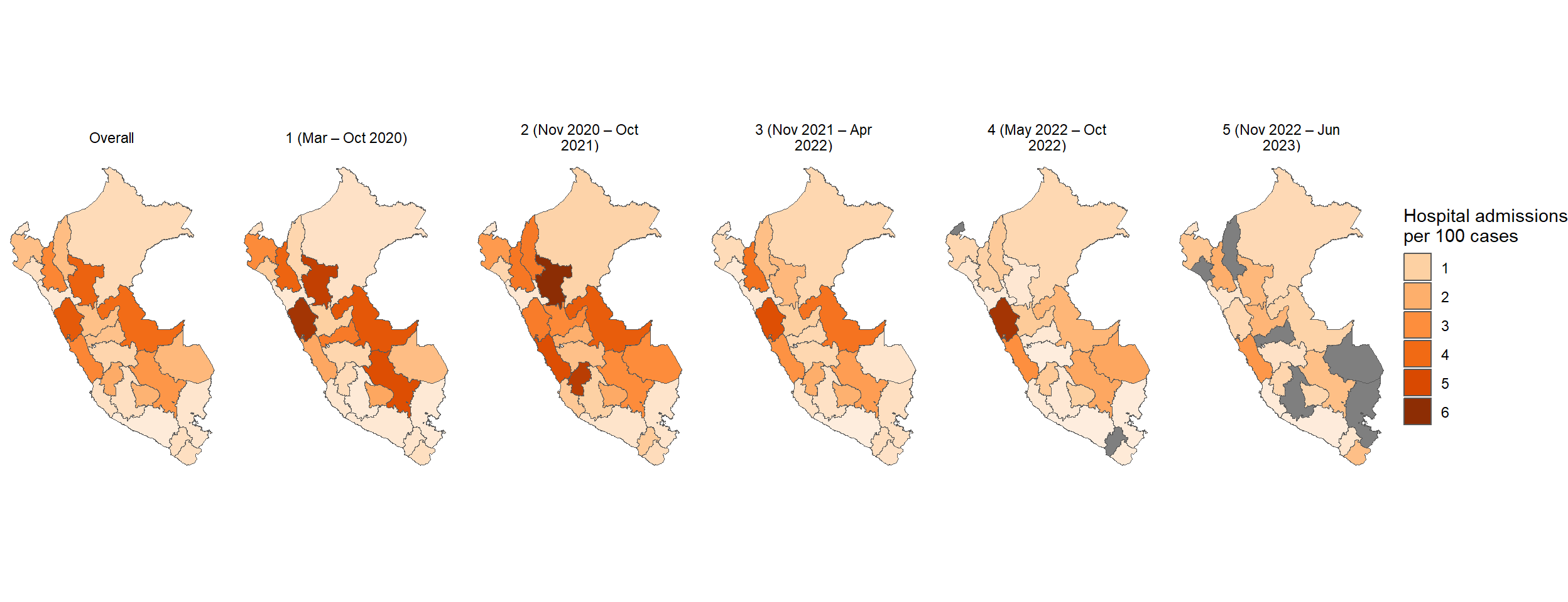
downloadthis::download_file(
  path = "02_output/tables/tasa_hospitalizacion_departamento.xlsx",
  button_label = "Descargar tabla en Excel",
  button_type = "success",
  has_icon = TRUE,
  icon = "fa fa-save"
)

In [238]:

downloadthis::download_file(
  path = "02_output/tables/tasa_hospitalizacion_departamento.docx",
  button_label = "Descargar tabla en Word",
  button_type = "primary",
  has_icon = TRUE,
  icon = "fa fa-save"
)

Departamento y Sexo

In [239]:

tasa_hospi_dep_sex_sf <- peru_dep_sf %>% 
  rename(departamento = dep) %>% 
  inner_join(
    results_hospi$departamento_sexo$index
  ) %>%
  ungroup()

Joining with `by = join_by(departamento)`

In [240]:

tasa_hospi_dep_sex_sf %>%
  ggplot() +
  geom_sf(aes(fill = rate)) +
  guides(
    fill = guide_legend(
      str_wrap(
        "Mean COVID-19 hospital admission rate per 100 COVID-19 cases",
        20
      )
    )
  ) +
  scale_fill_distiller(palette = "Oranges",  #"YlOrBr",
                       direction = 1) + 
  facet_wrap(vars(sexo)) + 
  theme_void()

Figura 33: Tasa de Hospitalización por 100 positivos COVID-19 de acuerdo al departamento y sexo(24-03-2020 a 16-06-2023)

In [241]:

results_hospi$departamento_sexo$index %>% 
  mutate(
    departamento = str_to_title(departamento),
    departamento = fct_reorder(departamento, rate, .desc = TRUE)
    # departamento = fct_reorder2(departamento, sexo, tasa_hospi_mes)
  ) %>%
  ggplot(aes(x = departamento, y = rate, fill = sexo)) +
  geom_bar(stat = "identity", position = position_dodge()) +
  theme_bw() +
  labs(title = "Hospital admissions COVID-19 by department and sex", 
       x = NULL, 
       y = "Mean COVID-19 hospital admission rate per 100 COVID-19 cases",
       fill = "Sex",
       caption = paste0("Total hospital admissions: ", 
                        scales::number(sum(pull(results_hospi$departamento_sexo$index_pre, count))))) +
  innovar::scale_fill_innova("blue_fall") +
  theme(
    axis.text.x = element_text(
      angle = 45,
      hjust = 1,
      vjust = 1
    )
  )

Figura 34: Tasa de Hospitalización por 100 positivos COVID-19 de acuerdo al departamento y sexo (24-03-2020 a 16-06-2023)

Departamento y Edad

In [242]:

tasa_hospi_dep_edad_sf <- peru_dep_sf %>% 
  rename(departamento = dep) %>% 
  inner_join(
    results_hospi$departamento_grupo_edad$index
  ) %>%
  ungroup()

Joining with `by = join_by(departamento)`

In [243]:

tasa_hospi_dep_edad_sf %>%
  ggplot() +
  geom_sf(aes(fill = rate)) +
  guides(
    fill = guide_legend(
      str_wrap(
        "Mean COVID-19 hospital admission rate per 100 COVID-19 cases",
        20
      )
    )
  ) +
  scale_fill_distiller(palette = "Oranges", # Old: "YlOrBr",
                       direction = 1) + 
  facet_wrap(vars(grupo_edad),
             nrow = 1) + 
  theme_void()

Figura 35: Tasa de Hospitalización por 100 positivos COVID-19 de acuerdo al departamento y grupo de edad(24-03-2020 a 16-06-2023)

Departamento y Olas

In [244]:

tasa_hospi_dep_olas_mother <- crossing(
  ola_covid = levels(results_hospi$departamento_ola_covid$index$ola_covid),
  departamento = unique(results_hospi$departamento_ola_covid$index$departamento)
)

tasa_hospi_dep_olas <- tasa_hospi_dep_olas_mother %>% 
  left_join(results_hospi$departamento_ola_covid$index) %>% 
  bind_rows(
    results_hospi$departamento$index %>% 
      mutate(ola_covid = "Overall")
  ) %>% 
  mutate(
    ola_covid = fct_recode(
      ola_covid,
      "1st wave" = "1 (Mar – Oct 2020)",
      "2nd wave" = "2 (Nov 2020 – Oct 2021)",
      "3rd wave" = "3 (Nov 2021 – Apr 2022)",
      "4th wave" = "4 (May 2022 – Oct 2022)",
      "5th wave" = "5 (Nov 2022 – Jun 2023)"
    ),
    ola_covid = fct_relevel(ola_covid,
                            "Overall")
  ) %>% 
  arrange(ola_covid)

Joining with `by = join_by(ola_covid, departamento)`

tasa_hospi_dep_olas_sf <- peru_dep_sf %>%
  rename(departamento = dep) %>% 
  left_join(
    tasa_hospi_dep_olas
  ) %>%
  ungroup()

Joining with `by = join_by(departamento)`

In [245]:

tasa_hospi_dep_olas_map <- tasa_hospi_dep_olas_sf %>%
  ggplot() +
  geom_sf(aes(fill = rate)) +
  guides(
    fill = guide_legend(
      str_wrap(
        "Mean COVID-19 hospital admission rate per 100 COVID-19 cases",
        20
      )
    )
  ) +
  scale_fill_distiller(palette = "Oranges", #Old: "YlOrBr",
                       direction = 1, na.value = "white") + 
  facet_wrap(vars(ola_covid), nrow = 1) + 
  theme_void()

tasa_hospi_dep_olas_map

Figura 36: Tasa de Hospitalización por 1000 positivos COVID-19 de acuerdo al departamento y ola (24-03-2020 a 16-06-2023)

Region

In [246]:

tasa_hospi_reg_sf <- peru_reg_sf %>% 
  inner_join(
    results_hospi$region$index
  )

Joining with `by = join_by(region)`

In [247]:

tasa_hospi_reg_map <- tasa_hospi_reg_sf %>%
  ggplot() +
  geom_sf(aes(fill = rate)) +
  guides(
    fill = guide_legend(
      str_wrap(
        "Mean COVID-19 hospital admission rate per 100 COVID-19 cases",
        20
      )
    )
  ) +
  ggsflabel::geom_sf_label(aes(label = region)) +
  scale_fill_distiller(palette = "Oranges", #Old: "YlOrBr",
                       direction = 1) + 
  theme_void()

tasa_hospi_reg_map

Warning in st_point_on_surface.sfc(data$geometry): st_point_on_surface may not
give correct results for longitude/latitude data

Figura 37: Tasa de Hospitalización por 100 positivos COVID-19 de acuerdo a la región (24-03-2020 a 16-06-2023)

Macrorregión

In [248]:

tasa_hospi_macro_sf <- peru_macro_sf %>% 
  inner_join(
    results_hospi$macrorregion$index
  )

Joining with `by = join_by(macrorregion)`

In [249]:

hospi_macro_map <- tasa_hospi_macro_sf %>%
  mutate(
    macrorregion = str_wrap(macrorregion, width = 15)
  ) %>%
  ggplot() +
  geom_sf(aes(fill = rate)) +
  ggsflabel::geom_sf_label_repel(aes(label = macrorregion),
                                 force = 100,
                                 seed = 2024) +
  guides(
    fill = guide_legend(
      str_wrap("Mean COVID-19 hospital admission rate per 100 COVID-19 cases", 
               20)
    )
  ) +
  scale_fill_distiller(palette = "Oranges", # Old: YlOrBr
                       direction = 1) + 
  theme_void()

hospi_macro_map

Warning in st_point_on_surface.sfc(data$geometry): st_point_on_surface may not
give correct results for longitude/latitude data

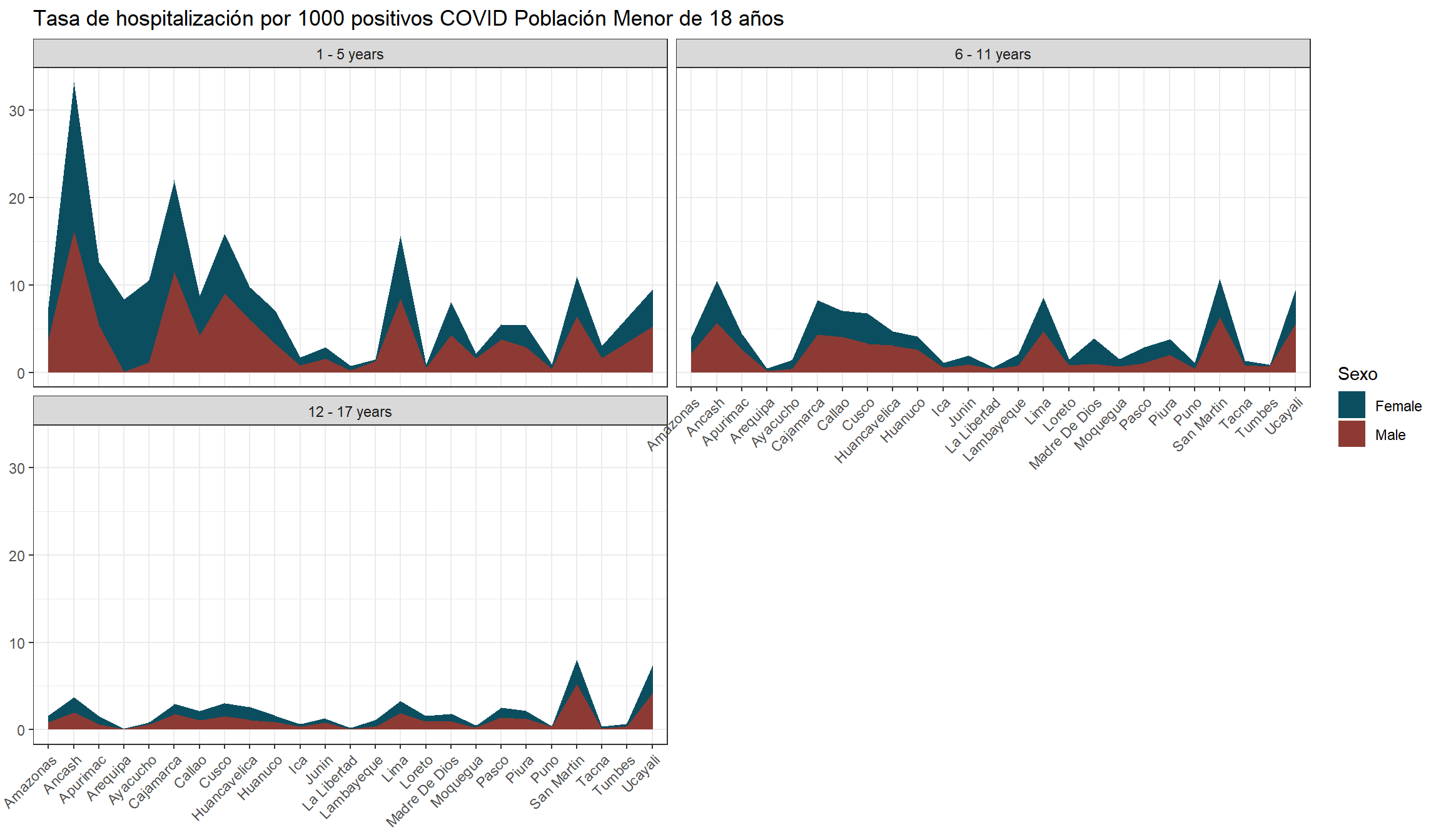
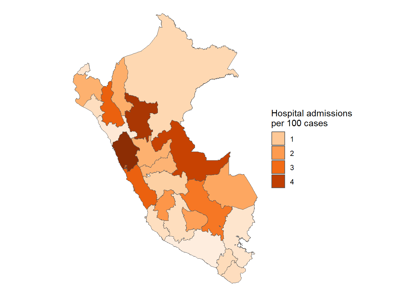
Figura 38: Tasa de Hospitalización por 1000 positivos COVID-19 de acuerdo a la macrorregión (24-03-2020 a 16-06-2023)

Distrital y pobreza

In [250]:

hospi_pobr_area_plot <- 
  results_per_month_hospi$cuartil_pobreza$index %>% 
  drop_na() %>% 
  mutate(
    time = make_date(anio, mes, "1")
  ) %>% 
  ggplot(
    aes(x = time,
        y = rate,
        fill = cuartil_pobreza)
  ) +
  geom_area(position = 'stack') +
  # innovar::scale_fill_innova("jama") +
  scale_fill_manual(
    values = c("#2C9BB4", "#0B4E60", "#DAE2BC", "#8C3A33")
  ) +
  scale_x_date(
    limits = c(ymd("2020-03-01"), ymd("2023-07-01")),
    breaks = seq(from = ceiling_date(ymd("2020-03-01"), "month"),
                 to = floor_date(ymd("2023-07-01"), "month"),
                 by = "2 months"), 
    # date_breaks = "2 month",
    date_labels = "%b %Y"
  ) +
  labs(
    y = NULL,
    x = NULL,
    title = "Monthly COVID-19 hospital admission",
    fill = "Poverty Quartiles"
  ) + 
  annotate(
    geom = "rect",
    xmin = as.Date("2020-03-01"), 
    xmax = as.Date("2020-10-31"), 
    ymin = 0, # El rectángulo se extiende hasta la parte inferior del gráfico
    ymax = Inf, # El rectángulo se extiende hasta la parte superior del gráfico
    color = "black", # Color de la línea
    fill = NA, # Sin relleno
    linetype = "dashed", # Tipo de línea discontinua
    linewidth = 0.5 # Grosor de la línea
  ) + 
  annotate(
    geom = "text", 
    x = as.Date("2020-07-01"), # Punto medio aproximado de la Ola 2
    y = Inf, # Posición vertical del texto
    label = "First wave", 
    color = "black",
    size = 4, # Tamaño del texto
    vjust = 2 # Ajuste vertical para colocar el texto encima del rectángulo
  ) +
  annotate(
    geom = "rect",
    xmin = as.Date("2020-11-01"), 
    xmax = as.Date("2021-10-31"), 
    ymin = 0, # El rectángulo se extiende hasta la parte inferior del gráfico
    ymax = Inf, # El rectángulo se extiende hasta la parte superior del gráfico
    color = "black", # Color de la línea
    fill = NA, # Sin relleno
    linetype = "dashed", # Tipo de línea discontinua
    linewidth = 0.5 # Grosor de la línea
  ) + 
  annotate(
    geom = "text", 
    x = as.Date("2021-05-10"), # Punto medio aproximado de la Ola 2
    y = Inf, # Posición vertical del texto
    label = "Second wave", 
    color = "black",
    size = 4, # Tamaño del texto
    vjust = 2 # Ajuste vertical para colocar el texto encima del rectángulo
  ) + 
  annotate(
    geom = "rect",
    xmin = as.Date("2021-11-01"), 
    xmax = as.Date("2022-04-30"), 
    ymin = 0, # El rectángulo se extiende hasta la parte inferior del gráfico
    ymax = Inf, # El rectángulo se extiende hasta la parte superior del gráfico
    color = "black", # Color de la línea
    fill = NA, # Sin relleno
    linetype = "dashed", # Tipo de línea discontinua
    linewidth = 0.5 # Grosor de la línea
  ) + 
  annotate(
    geom = "text", 
    x = as.Date("2022-02-01"), # Punto medio aproximado de la Ola 2
    y = Inf, # Posición vertical del texto
    label = "Third \nwave", 
    color = "black",
    size = 4, # Tamaño del texto
    vjust = 1.25 # Ajuste vertical para colocar el texto encima del rectángulo
  ) + 
  annotate(
    geom = "rect",
    xmin = as.Date("2022-05-01"), 
    xmax = as.Date("2022-10-31"), 
    ymin = 0, # El rectángulo se extiende hasta la parte inferior del gráfico
    ymax = Inf, # El rectángulo se extiende hasta la parte superior del gráfico
    color = "black", # Color de la línea
    fill = NA, # Sin relleno
    linetype = "dashed", # Tipo de línea discontinua
    linewidth = 0.5 # Grosor de la línea
  ) + 
  annotate(
    geom = "text", 
    x = as.Date("2022-08-01"), # Punto medio aproximado de la Ola 2
    y = Inf, # Posición vertical del texto
    label = "Fourth \nwave", 
    color = "black",
    size = 4, # Tamaño del texto
    vjust = 1.25 # Ajuste vertical para colocar el texto encima del rectángulo
  ) +
  annotate(
    geom = "rect",
    xmin = as.Date("2022-11-01"), 
    xmax = as.Date("2023-07-01"), 
    ymin = 0, # El rectángulo se extiende hasta la parte inferior del gráfico
    ymax = Inf, # El rectángulo se extiende hasta la parte superior del gráfico
    color = "black", # Color de la línea
    fill = NA, # Sin relleno
    linetype = "dashed", # Tipo de línea discontinua
    linewidth = 0.5 # Grosor de la línea
  ) + 
  annotate(
    geom = "text", 
    x = as.Date("2023-03-01"),
    y = Inf, # Posición vertical del texto
    label = "Fifth wave", 
    color = "black",
    size = 4, # Tamaño del texto
    vjust = 2 # Ajuste vertical para colocar el texto encima del rectángulo
  ) +
  theme_classic() +
  theme(
    axis.text.x = element_text(
      angle = 75,
      vjust = 0.5
    ),
    axis.ticks.x = element_line()
  ) 

hospi_pobr_area_plot

Figura 39: Mortalidad COVID-19 de acuerdo al cuartil de pobreza(14-03-2020 a 13-06-2023)

Distrito Lima

In [251]:

total_hospi_distr_lim_callao <- results_hospi$distrito$index_pre %>% 
  filter(provincia %in% c("LIMA", "CALLAO")) %>% 
  pull(count) %>% 
  sum()

results_hospi$distrito$index %>% 
  filter(provincia %in% c("LIMA", "CALLAO")) %>% 
  drop_na() %>% 
  mutate(
    distrito = str_to_title(distrito), 
    distrito = fct_reorder(distrito, rate)
  ) %>% 
  ggplot(aes(y = distrito, x = rate)) +
  geom_bar(stat = "identity",
           color = "black",
           fill = "grey80") +
  theme_bw() +
  labs(title = "Hospital admissions COVID-19 in Metropolitan Lima", 
       x = NULL, 
       y = "Mean COVID-19 hospital admission rate per 100 COVID-19 cases",
       caption = paste0("Total hospital admissions: ", 
                        scales::number(total_hospi_distr_lim_callao))) +
  innovar::scale_fill_innova("blue_fall") +
  theme(
    legend.position = "bottom"
  )

Figura 40: Tasa de Hospitalización COVID-19 de acuerdo a los distritos de lima metropolitana (24-03-2020 a 16-06-2023)

In [252]:

tasa_hospi_lima_distr_1k_sf <- Peru %>% 
  inner_join(
    results_hospi$distrito$index %>% 
      filter(provincia %in% c("LIMA", "CALLAO"))
  )

Joining with `by = join_by(ubigeo)`

In [253]:

tasa_hospi_lima_distr_1k_sf %>%
  mutate(
    label = case_when(
      rate > 25 ~ str_to_title(distrito)
    )
  ) %>%
  ggplot() +
  geom_sf(aes(fill = rate)) +
  guides(
    fill = guide_legend(
      str_wrap("Mean COVID-19 hospital admission rate per 100 COVID-19 cases", 
               20)
    )
  ) +
  ggsflabel::geom_sf_label_repel(aes(label = label),
                                 force = 10,
                                 size = 2.45,
                                 box.padding = 0.75,
                                 seed = 2024) +
  scale_fill_distiller(palette = "YlOrBr",
                       direction = 1) + 
  theme_void()

Warning in st_point_on_surface.sfc(data$geometry): st_point_on_surface may not
give correct results for longitude/latitude data

Warning: Removed 48 rows containing missing values or values outside the scale range
(`geom_label_repel()`).

Figura 41: Tasa de Hospitalización COVID-19 de acuerdo a los distritos de lima metropolitana (24-03-2020 a 16-06-2023)

In [254]:

In [255]:

tbl_summ_tasa_hospi_lima_distr_pre <- results_hospi$distrito$index %>% 
      filter(provincia %in% c("LIMA", "CALLAO")) %>% 
  mutate(
    across(
      departamento:distrito,
      str_to_title
    ),
    rate = formattable::digits(rate, 3)
  ) %>% 
  select(-departamento)

tbl_summ_tasa_hospi_lima_distr <- tbl_summ_tasa_hospi_lima_distr_pre %>% 
  rename_with(
    .fn = ~ paste0("**", str_to_title(.x), "**")
  ) %>% 
  gt::gt() %>% 
  gt::cols_label(
    .fn = gt::md,
    .process_units = TRUE
  )

tbl_summ_tasa_hospi_lima_distr

Tabla 30: Tasa de Hospitalización COVID-19 de acuerdo a los distritos de lima metropolitana (24-03-2020 a 16-06-2023)

Ubigeo	Provincia	Distrito	Rate
070101	Callao	Callao	2.327
070102	Callao	Bellavista	0.870
070103	Callao	Carmen De La Legua Reynoso	NA
070104	Callao	La Perla	0.937
070106	Callao	Ventanilla	3.471
070107	Callao	Mi Peru	3.256
150101	Lima	Lima	3.184
150102	Lima	Ancon	4.301
150103	Lima	Ate	2.615
150104	Lima	Barranco	0.951
150105	Lima	Brena	16.426
150106	Lima	Carabayllo	2.786
150107	Lima	Chaclacayo	0.620
150108	Lima	Chorrillos	1.923
150109	Lima	Cieneguilla	3.906
150110	Lima	Comas	2.839
150111	Lima	El Agustino	1.860
150112	Lima	Independencia	5.366
150113	Lima	Jesus Maria	0.384
150114	Lima	La Molina	0.292
150115	Lima	La Victoria	2.023
150116	Lima	Lince	1.149
150117	Lima	Los Olivos	3.042
150118	Lima	Lurigancho	2.291
150119	Lima	Lurin	14.056
150120	Lima	Magdalena Del Mar	0.251
150121	Lima	Pueblo Libre	0.496
150122	Lima	Miraflores	0.357
150123	Lima	Pachacamac	7.502
150124	Lima	Pucusana	13.415
150125	Lima	Puente Piedra	5.234
150126	Lima	Punta Hermosa	13.253
150127	Lima	Punta Negra	6.098
150128	Lima	Rimac	7.053
150129	Lima	San Bartolo	9.821
150130	Lima	San Borja	1.491
150131	Lima	San Isidro	0.195
150132	Lima	San Juan De Lurigancho	4.658
150133	Lima	San Juan De Miraflores	3.851
150134	Lima	San Luis	1.077
150135	Lima	San Martin De Porres	5.082
150136	Lima	San Miguel	0.787
150137	Lima	Santa Anita	2.585
150138	Lima	Santa Maria Del Mar	5.263
150139	Lima	Santa Rosa	6.742
150140	Lima	Santiago De Surco	0.482
150141	Lima	Surquillo	1.001
150142	Lima	Villa El Salvador	31.365
150143	Lima	Villa Maria Del Triunfo	7.358

In [256]:

tbl_summ_tasa_hospi_lima_distr_pre %>% 
  rename_with(
    .fn = str_to_title
  ) %>% 
  huxtable::as_hux() %>% 
  huxtable::set_bold(1, 1:4) %>% 
  huxtable::quick_xlsx(file = "02_output/tables/tasa_hospitalizacion_lima_distrito.xlsx",
                       open = FALSE)

tbl_summ_tasa_hospi_lima_distr %>%
  gt::gtsave("02_output/tables/tasa_hospitalizacion_lima_distrito.docx")

In [257]:

downloadthis::download_file(
  path = "02_output/tables/tasa_hospitalizacion_lima_distrito.xlsx",
  button_label = "Descargar tabla en Excel",
  button_type = "success",
  has_icon = TRUE,
  icon = "fa fa-save"
)

In [258]:

downloadthis::download_file(
  path = "02_output/tables/tasa_hospitalizacion_lima_distrito.docx",
  button_label = "Descargar tabla en Word",
  button_type = "primary",
  has_icon = TRUE,
  icon = "fa fa-save"
)

Tasa de Vacunación

In [259]:

vacunas_18 <- vacunas_18 %>% 
  filter(dosis %in% 1:3) %>% 
  mutate(
    overall = "overall"
  ) 

range_vacu <- vacunas_18 %>% 
  summarise(
    min = min(fecha_vacunacion),
    max = max(fecha_vacunacion)
  ) %>% 
  collect() %>% 
  mutate(
    min = format(min, "%d-%m-%Y"),
    max = format(max, "%d-%m-%Y"),
    fecha = paste0("(", min, " a ", max, ")")
  )

Vista General

Cálculo de tasa de vacunación

In [260]:

levels <- list(
  c("overall"),
  c("dosis"),
  c("grupo_edad"),
  c("sexo"),
  c("ola_covid"),
  c("ola_covid", "grupo_edad"),
  c("departamento"),
  c("departamento", "sexo"),
  c("departamento", "grupo_edad"),
  c("departamento", "sexo", "grupo_edad"),
  c("departamento", "ola_covid"),
  c("distrito"),
  c("distrito", "sexo"),
  c("distrito", "grupo_edad"),
  c("distrito", "cuartil_pobreza"),
  c("grupo_edad", "cuartil_pobreza"),
  c("sexo", "cuartil_pobreza"),
  c("ola_covid", "cuartil_pobreza"),
  c("cuartil_pobreza"),
  c("ola_covid", "cuartil_nbi"),
  c("cuartil_nbi"),
  c("region"),
  c("region", "grupo_edad"),
  c("macrorregion"),
  c("macrorregion", "grupo_edad"),
  c("grupo_edad", "dosis"),
  c("sexo", "dosis"),
  c("ola_covid", "sexo"),
  c("ola_covid", "region"),
  c("ola_covid", "macrorregion"),
  c("ola_covid", "dosis"),
  c("ola_covid", "grupo_edad", "dosis"),
  c("departamento", "dosis"),
  c("departamento", "sexo", "dosis"),
  c("departamento", "grupo_edad", "dosis"),
  c("departamento", "sexo", "grupo_edad", "dosis"),
  c("departamento", "ola_covid", "dosis"),
  c("distrito", "dosis"),
  c("distrito", "sexo", "dosis"),
  c("distrito", "grupo_edad", "dosis"),
  c("distrito", "cuartil_pobreza", "dosis"),
  c("grupo_edad", "cuartil_pobreza", "dosis"),
  c("sexo", "cuartil_pobreza", "dosis"),
  c("ola_covid", "cuartil_pobreza", "dosis"),
  c("cuartil_pobreza", "dosis"),
  c("cuartil_nbi", "dosis"),
  c("region", "dosis"),
  c("region", "grupo_edad", "dosis"),
  c("macrorregion", "dosis"),
  c("macrorregion", "grupo_edad", "dosis")
)

# Calcular la tasa de vacunacion
results_vacunas <- index_calculator(
  data = vacunas_18, 
  denom = poblacion %>% mutate(overall = "overall"), 
  levels = levels, 
  type = "month"
)

# Calcular la tasa de vacunacion
results__per_month_vacunas <- index_calculator(
  data = vacunas_18, 
  denom = poblacion %>% mutate(overall = "overall"), 
  levels = levels, 
  type = "per_month"
)

In [261]:

vacunas_18_descr_tbl <- vacunas_18 %>% 
  select(edad, overall, grupo_edad, sexo, ola_covid, region, 
         macrorregion, cuartil_pobreza, cuartil_nbi,
         dosis) %>% 
  collect() 

labelled::var_label(vacunas_18_descr_tbl) <- list(
  overall = "Overall",
  grupo_edad = "Age Group",
  sexo = "Sex",
  ola_covid = "COVID-19 wave",
  region = "Natural Regions",
  macrorregion = "Macroregions",
  cuartil_pobreza = "Poverty level",
  cuartil_nbi = "Unsatisfied basic needs level",
  dosis = "Doses"
)

In [262]:

tbl_summ_vacunas_g <- vacunas_18_descr_tbl %>% 
  select(-edad) %>% 
  gtsummary::tbl_summary(
    type = list(
      overall ~ "dichotomous"
    ),
    value = list(overall = "overall"),
    missing_text = "No data"
  ) %>% 
  gtsummary::modify_header(label = "**Variables**") %>%
  gtsummary::bold_labels()


tbl_summ_vacunas_c2 <- results_vacunas$overall$index %>% 
  mutate(label = "Overall") %>% 
  rename(variable = overall) %>% 
  bind_rows(
    results_vacunas$grupo_edad$index %>% 
      mutate(variable = "grupo_edad") %>% 
      rename(label = grupo_edad),
    results_vacunas$sexo$index %>% 
      mutate(variable = "sexo") %>% 
      rename(label = sexo),
    results_vacunas$ola_covid$index %>% 
      mutate(variable = "ola_covid") %>% 
      rename(label = ola_covid),
    results_vacunas$region$index %>% 
      mutate(variable = "region") %>% 
      rename(label = region),
    results_vacunas$macrorregion$index %>% 
      mutate(variable = "macrorregion") %>% 
      rename(label = macrorregion),
    results_vacunas$cuartil_pobreza$index %>% 
      mutate(variable = "cuartil_pobreza") %>% 
      rename(label = cuartil_pobreza),
    results_vacunas$cuartil_nbi$index %>% 
      mutate(variable = "cuartil_nbi") %>% 
      rename(label = cuartil_nbi),
    results_vacunas$dosis$index %>% 
      mutate(dosis = as.character(dosis),
             variable = "dosis") %>% 
      rename(label = dosis)
  ) %>% 
  drop_na() %>% 
  mutate(
    rate = formattable::digits(rate, 3)
  )

tbl_summ_vacunas_final <- tbl_summ_vacunas_g %>%
  gtsummary::modify_table_body(
    ~ .x %>% 
      left_join(tbl_summ_vacunas_c2) %>% 
      mutate(
        label = case_when(
          variable %in% c("cuartil_pobreza", "cuartil_nbi") &
            label == "1" ~ "1 (0-19.9%)",
          variable %in% c("cuartil_pobreza", "cuartil_nbi") & 
            label == "2" ~ "2 (20-39.9%)",
          variable %in% c("cuartil_pobreza", "cuartil_nbi") & 
            label == "3" ~ "3 (40-59.9%)",
          variable %in% c("cuartil_pobreza", "cuartil_nbi") &
            label == "4" ~ "4 (60-100%)",
          .default = label
        )
      )
  ) %>% 
  gtsummary::modify_header(
    rate ~ "**Vaccine dose rate per 1,000 inhabitants**"
  ) %>%
  gtsummary::modify_fmt_fun(
    rate ~ scales::number_format(accuracy = 0.001)
  )

Joining with `by = join_by(variable, label)`

In [263]:

tbl_summ_vacunas_final

Tabla 31: Descriptivos de vacunación menores de 18 años (03-01-2021 a 17-06-2023)

Variables	N = 16,440,145¹	Vaccine dose rate per 1,000 inhabitants
Overall	16,440,145 (100%)	55.895
Age Group
Under 1 year	1,197 (<0.1%)	0.129
1 - 5 years	1,551,218 (9.4%)	19.696
6 - 11 years	6,497,774 (40%)	69.704
12 - 17 years	8,389,956 (51%)	83.420
Sex
Female	8,274,543 (50%)	58.273
Male	8,165,602 (50%)	55.469
COVID-19 wave
1 (Mar – Oct 2020)	0 (0%)
2 (Nov 2020 – Oct 2021)	624,089 (3.8%)	6.055
3 (Nov 2021 – Apr 2022)	11,485,397 (70%)	194.523
4 (May 2022 – Oct 2022)	3,159,814 (19%)	55.161
5 (Nov 2022 – Jun 2023)	1,170,845 (7.1%)	14.774
Natural Regions
Coast	10,929,273 (66%)	61.803
Highlands	3,816,009 (23%)	47.822
Jungle	1,694,863 (10%)	51.057
Macroregions
Center	3,807,667 (23%)	60.850
East	1,623,558 (9.9%)	51.312
Metropolitan Lima and Callao	4,992,488 (30%)	61.590
North	3,914,033 (24%)	60.102
South	2,102,399 (13%)	45.287
Poverty level
1 (0-19.9%)	10,203,044 (62%)	61.242
2 (20-39.9%)	4,175,432 (25%)	54.832
3 (40-59.9%)	1,680,893 (10%)	45.605
4 (60-100%)	376,414 (2.3%)	49.542
No data	4,362
Unsatisfied basic needs level
1 (0-19.9%)	7,820,622 (48%)	60.664
2 (20-39.9%)	5,937,285 (36%)	59.327
3 (40-59.9%)	1,846,848 (11%)	48.271
4 (60-100%)	831,028 (5.1%)	41.112
No data	4,362
Doses
1	7,457,839 (45%)	25.228
2	6,341,776 (39%)	22.241
3	2,640,530 (16%)	9.823
¹ n (%)

In [264]:

tbl_summ_vacunas_final %>% 
  gtsummary::as_hux_xlsx("02_output/tables/vacunas_descriptivos.xlsx")

tbl_summ_vacunas_final %>%
  gtsummary::as_flex_table() %>%
  flextable::save_as_docx(path = "02_output/tables/vacunas_descriptivos.docx")

In [265]:

downloadthis::download_file(
  path = "02_output/tables/vacunas_descriptivos.xlsx",
  button_label = "Descargar tabla en Excel",
  button_type = "success",
  has_icon = TRUE,
  icon = "fa fa-save"
)

In [266]:

downloadthis::download_file(
  path = "02_output/tables/vacunas_descriptivos.docx",
  button_label = "Descargar tabla en Word",
  button_type = "primary",
  has_icon = TRUE,
  icon = "fa fa-save"
)

In [267]:

comparing_levels <- list(
  c("grupo_edad"),
  c("sexo"),
  c("ola_covid"),
  c("cuartil_pobreza"),
  c("cuartil_nbi"),
  c("region"),
  c("macrorregion")
)

vacunas_comparisons <- compare_levels_per_month(
  results_per_month = results__per_month_vacunas,
  levels = comparing_levels
)

# Extraer las tablas `cld` como tibbles, renombrando y añadiendo una columna "level"
vacunas_comparisons_cld_pre <- lapply(names(vacunas_comparisons), function(level) {
  cld <- vacunas_comparisons[[level]]$cld
  
  if (!is.null(cld)) {
    cld <- cld |> 
      as_tibble() |> 
      rename(group = 1) |>  # Renombra la primera columna a 'group'
      mutate(level = level) |> # Añade una columna 'level' con el nombre de la lista
      relocate(level) 
  }
  
  cld
}) |> 
  bind_rows()

vacunas_comparisons_cld_pre <- 
  vacunas_comparisons_cld_pre |> 
  mutate(
    across(
      where(is.numeric),
      ~ formattable::digits(.x, 3)
    )
  )

In [268]:

In [269]:

vacunas_comparisons_cld <- vacunas_comparisons_cld_pre |> 
  rename_with(
    .fn = ~ paste0("**", str_to_title(.x), "**")
  ) %>% 
  gt::gt() %>% 
  gt::cols_label(
    .fn = gt::md,
    .process_units = TRUE
  )

vacunas_comparisons_cld

Tabla 32: Comparaciones múltiples de vacunas(07-03-2020 a 17-06-2023)

Level	Group	Emmean	Se	Df	Lower.cl	Upper.cl	.Group
grupo_edad	Under 1 year	-1.850	30.199	100.999	-61.757	58.056	a
grupo_edad	1 - 5 years	19.599	23.137	100.760	-26.299	65.497	a
grupo_edad	6 - 11 years	69.607	23.137	100.760	23.709	115.506	a
grupo_edad	12 - 17 years	83.420	22.748	100.746	38.292	128.548	a
sexo	Male	55.469	14.992	29.007	24.806	86.132	a
sexo	Female	56.361	14.993	29.008	25.698	87.024	b
ola_covid	2 (Nov 2020 – Oct 2021)	6.055	12.693	26.000	-20.037	32.146	a
ola_covid	5 (Nov 2022 – Jun 2023)	14.774	14.192	26.000	-14.397	43.945	a
ola_covid	4 (May 2022 – Oct 2022)	55.161	16.387	26.000	21.477	88.845	a
ola_covid	3 (Nov 2021 – Apr 2022)	194.523	16.387	26.000	160.839	228.207	b
cuartil_pobreza	3	43.713	13.505	34.298	16.277	71.149	a
cuartil_pobreza	4	43.757	13.575	34.985	16.198	71.317	a
cuartil_pobreza	2	52.940	13.505	34.298	25.504	80.376	ab
cuartil_pobreza	1	61.242	13.459	33.876	33.887	88.598	b
cuartil_nbi	4	39.234	13.764	34.215	11.268	67.200	a
cuartil_nbi	3	46.392	13.764	34.215	18.426	74.358	ab
cuartil_nbi	2	57.448	13.764	34.215	29.482	85.414	b
cuartil_nbi	1	60.664	13.719	33.801	32.779	88.550	b
region	Highlands	45.855	14.347	32.398	16.646	75.064	a
region	Jungle	49.090	14.347	32.398	19.881	78.299	ab
region	Coast	61.803	14.310	32.093	32.658	90.949	b
macrorregion	South	43.311	14.939	32.683	12.906	73.716	a
macrorregion	East	49.335	14.939	32.683	18.930	79.740	ab
macrorregion	North	58.125	14.939	32.683	27.720	88.530	ab
macrorregion	Center	58.873	14.939	32.683	28.468	89.278	ab
macrorregion	Metropolitan Lima and Callao	61.590	14.905	32.399	31.245	91.936	b

In [270]:

vacunas_comparisons_cld_pre %>% 
  rename_with(
    .fn = str_to_title
  ) %>% 
  huxtable::as_hux() %>% 
  huxtable::set_bold(1, 1:8) %>% 
  huxtable::quick_xlsx(file = "02_output/tables/vacunas_comparacion_multiple.xlsx",
                       open = FALSE)

vacunas_comparisons_cld %>%
  gt::gtsave("02_output/tables/vacunas_comparacion_multiple.docx")

In [271]:

downloadthis::download_file(
  path = "02_output/tables/vacunas_comparacion_multiple.xlsx",
  button_label = "Descargar tabla en Excel",
  button_type = "success",
  has_icon = TRUE,
  icon = "fa fa-save"
)

In [272]:

downloadthis::download_file(
  path = "02_output/tables/vacunas_comparacion_multiple.docx",
  button_label = "Descargar tabla en Word",
  button_type = "primary",
  has_icon = TRUE,
  icon = "fa fa-save"
)

In [273]:

tbl_summ_vacunas_olas <- vacunas_18_descr_tbl %>% 
  select(-edad) %>% 
  gtsummary::tbl_summary(
    by = ola_covid,
    type = list(
      overall ~ "dichotomous"
    ),
    value = list(overall = "overall"),
    missing_text = "No data"
  ) %>% 
  gtsummary::modify_header(label = "**Variables**") %>%
  gtsummary::bold_labels()

ola_covid_vacunas_gtsumm <- results_vacunas$ola_covid$index %>% 
  rename(stat = ola_covid) %>% 
  mutate(label = "Overall",
         variable = "overall") %>% 
  bind_rows(
    results_vacunas$ola_covid_grupo_edad$index %>%
      mutate(variable = "grupo_edad") %>% 
      rename(label = grupo_edad,
             stat = ola_covid),
    results_vacunas$ola_covid_sexo$index %>% 
      mutate(variable = "sexo") %>% 
      rename(label = sexo,
             stat = ola_covid),
    results_vacunas$ola_covid_region$index %>% 
      mutate(variable = "region") %>% 
      rename(label = region,
             stat = ola_covid),
    results_vacunas$ola_covid_macrorregion$index %>% 
      mutate(variable = "macrorregion") %>%
      rename(label = macrorregion,
             stat = ola_covid),
    results_vacunas$ola_covid_cuartil_pobreza$index %>% 
      mutate(variable = "cuartil_pobreza") %>% 
      rename(label = cuartil_pobreza,
             stat = ola_covid),
    results_vacunas$ola_covid_cuartil_nbi$index %>% 
      mutate(variable = "cuartil_nbi") %>% 
      rename(label = cuartil_nbi,
             stat = ola_covid),
    results_vacunas$ola_covid_dosis$index %>% 
      mutate(dosis = as.character(dosis),
             variable = "dosis") %>% 
      rename(label = dosis,
             stat = ola_covid)
  ) %>% 
  mutate(
    rate = formattable::digits(rate, 3),
    stat = as.character(stat),
    stat = case_match(
      stat,
      "1 (Mar – Oct 2020)" ~ "stat_1",
      "2 (Nov 2020 – Oct 2021)" ~ "stat_2",
      "3 (Nov 2021 – Apr 2022)" ~ "stat_3",
      "4 (May 2022 – Oct 2022)" ~ "stat_4",
      "5 (Nov 2022 – Jun 2023)" ~ "stat_5"
    )
  ) 

tbl_summ_vacunas_olas$table_body <- tbl_summ_vacunas_olas$table_body %>%
  mutate(
    across(
      gtsummary::all_stat_cols(stat_0 = FALSE),
      ~ str_remove_all(., "\\s*\\(.*?\\)\\s*")
    )
  ) %>% 
  pivot_longer(
    cols = stat_1:stat_5,
    names_to = "stat",
    values_to = "freq"
  ) %>% 
  left_join(
    ola_covid_vacunas_gtsumm
  ) %>% 
  mutate(
    value = str_c(freq, ifelse(is.na(rate), "", str_c(" (", rate, ")")))
  ) %>% 
  select(-c(freq, rate)) %>% 
  pivot_wider(
    names_from = stat,
    values_from = value
  )

Joining with `by = join_by(variable, label, stat)`

In [274]:

tbl_summ_vacunas_olas <- tbl_summ_vacunas_olas %>% 
  gtsummary::modify_footnote(
    gtsummary::all_stat_cols() ~ "n (Vaccine dose rate per 1,000 inhabitants)"
  )

tbl_summ_vacunas_olas

Tabla 33: Descriptivos de vacunación menores de 18 años por olas (03-01-2021 a 17-06-2023)

Variables	1 (Mar – Oct 2020) N = 0¹	2 (Nov 2020 – Oct 2021) N = 624,089¹	3 (Nov 2021 – Apr 2022) N = 11,485,397¹	4 (May 2022 – Oct 2022) N = 3,159,814¹	5 (Nov 2022 – Jun 2023) N = 1,170,845¹
Overall	0	624,089 (6.055)	11,485,397 (194.523)	3,159,814 (55.161)	1,170,845 (14.774)
Age Group
Under 1 year	0	869 (0.172)	325 (0.105)	3 (0.003)	0
1 - 5 years	0	186 (0.007)	669,736 (40.901)	301,108 (18.389)	580,188 (26.922)
6 - 11 years	0	1,921 (0.062)	4,863,069 (253.116)	1,215,863 (63.292)	416,921 (15.303)
12 - 17 years	0	621,113 (17.799)	5,952,267 (291.382)	1,642,840 (87.311)	173,736 (6.556)
Sex
Female	0	319,569 (6.788)	5,752,001 (194.600)	1,610,222 (56.665)	592,751 (15.155)
Male	0	304,520 (5.999)	5,733,396 (194.462)	1,549,592 (53.680)	578,094 (14.403)
Natural Regions
Coast	0	434,934 (7.062)	7,791,974 (220.072)	1,943,551 (56.447)	758,814 (15.546)
Highlands	0	181,258 (6.545)	2,532,616 (151.066)	819,090 (51.827)	283,045 (13.824)
Jungle	0	7,897 (0.819)	1,160,807 (171.501)	397,173 (56.355)	128,986 (13.269)
Macroregions
Center	0	130,600 (6.142)	2,519,235 (192.206)	846,044 (67.755)	311,788 (18.701)
East	0	7,857 (0.853)	1,112,025 (172.244)	378,698 (56.416)	124,978 (13.549)
Metropolitan Lima and Callao	0	119,044 (4.071)	3,749,618 (230.373)	783,267 (50.570)	340,559 (15.168)
North	0	144,791 (7.057)	2,742,763 (203.584)	748,123 (56.098)	278,356 (15.169)
South	0	221,797 (14.350)	1,361,756 (141.439)	403,682 (43.595)	115,164 (9.248)
Poverty level
1	0	523,019 (9.530)	7,216,622 (217.375)	1,835,414 (54.987)	627,989 (13.475)
2	0	79,590 (3.161)	2,912,849 (183.582)	848,412 (55.497)	334,581 (15.901)
3	0	17,460 (1.157)	1,100,108 (137.405)	395,854 (57.159)	167,471 (18.094)
4	0	3,483 (1.444)	252,952 (144.811)	79,357 (50.759)	40,622 (19.264)
No data	0	537	2,866	777	182
Unsatisfied basic needs level
1	0	448,134 (10.420)	5,546,126 (215.620)	1,348,320 (52.529)	478,042 (13.355)
2	0	137,619 (4.134)	4,158,423 (199.297)	1,182,153 (59.028)	459,090 (16.666)
3	0	25,548 (1.858)	1,247,998 (154.133)	419,836 (56.330)	153,466 (15.044)
4	0	12,251 (1.745)	529,984 (124.635)	208,728 (52.083)	80,065 (14.530)
No data	0	537	2,866	777	182
Doses
1	0	539,332 (5.233)	5,964,066 (101.031)	500,204 (8.732)	454,237 (5.742)
2	0	84,696 (0.913)	5,244,815 (88.669)	710,017 (12.395)	302,248 (3.797)
3	0	61 (0.001)	276,516 (4.824)	1,949,593 (34.034)	414,360 (5.235)
¹ n (Vaccine dose rate per 1,000 inhabitants)

In [275]:

tbl_summ_vacunas_olas %>% 
  gtsummary::as_hux_xlsx("02_output/tables/vacunas_olas_descriptivos.xlsx")

tbl_summ_vacunas_olas %>%
  gtsummary::as_flex_table() %>%
  flextable::save_as_docx(path = "02_output/tables/vacunas_olas_descriptivos.docx")

In [276]:

downloadthis::download_file(
  path = "02_output/tables/fallecidos_olas_descriptivos.xlsx",
  button_label = "Descargar tabla en Excel",
  button_type = "success",
  has_icon = TRUE,
  icon = "fa fa-save"
)

In [277]:

downloadthis::download_file(
  path = "02_output/tables/fallecidos_olas_descriptivos.docx",
  button_label = "Descargar tabla en Word",
  button_type = "primary",
  has_icon = TRUE,
  icon = "fa fa-save"
)

Gráfico de vacunación (serie de tiempo) - Menores de 18 años

Se restringió la visualización de dosis de 1 a 5.

In [278]:

summ_vacunas_dosis_fecha <- vacunas_18 %>% 
  to_arrow() %>%
  mutate(
    fecha_round = ceiling_date(fecha_vacunacion, unit = "month"),
    .after = fecha_vacunacion
  ) %>%
  # filter(dosis %in% 1:5) %>% 
  count(dosis, fecha_round) %>% 
  collect()

summ_vacunas_dosis_fecha %>% 
  ggplot(
    aes(
      x = fecha_round,
      y = n,
      fill = as.factor(dosis)
    )
  ) +
  geom_area(position = 'stack') +
  scale_fill_manual(
    values = c("#2C9BB4", "#0B4E60", "#8C3A33")
  ) +
  # scale_x_date(
  #   limits = c(ymd("2020-03-01"), ymd("2023-10-31")),
  #   breaks = scales::date_breaks("2 month"), # Cambiar a "6 months" para menos frecuencia
  #   labels = scales::date_format("%b %Y") # Formato de fecha, %b es la abreviatura de mes, %Y es el año
  # ) + 
  scale_x_date(
    limits = c(ymd("2020-03-01"), ymd("2023-07-01")),
    breaks = seq(from = ceiling_date(ymd("2020-03-01"), "month"),
                 to = floor_date(ymd("2023-07-01"), "month"),
                 by = "2 months"), 
    # date_breaks = "2 month",
    date_labels = "%b %Y"
  ) +
  scale_y_continuous(
    labels = scales::number_format()
  ) +
  labs(
    y = NULL,
    x = NULL,
    title = "Vaccination COVID-19 under 18 years old",
    fill = "Doses"
  ) + 
  annotate(
    geom = "rect",
    xmin = as.Date("2020-03-01"), 
    xmax = as.Date("2020-10-31"), 
    ymin = 0, # El rectángulo se extiende hasta la parte inferior del gráfico
    ymax = Inf, # El rectángulo se extiende hasta la parte superior del gráfico
    color = "black", # Color de la línea
    fill = NA, # Sin relleno
    linetype = "dashed", # Tipo de línea discontinua
    linewidth = 0.5 # Grosor de la línea
  ) + 
  annotate(
    geom = "text", 
    x = as.Date("2020-07-01"), # Punto medio aproximado de la Ola 2
    y = Inf, # Posición vertical del texto
    label = "First wave", 
    color = "black",
    size = 4, # Tamaño del texto
    vjust = 2 # Ajuste vertical para colocar el texto encima del rectángulo
  ) +
  annotate(
    geom = "rect",
    xmin = as.Date("2020-11-01"), 
    xmax = as.Date("2021-10-31"), 
    ymin = 0, # El rectángulo se extiende hasta la parte inferior del gráfico
    ymax = Inf, # El rectángulo se extiende hasta la parte superior del gráfico
    color = "black", # Color de la línea
    fill = NA, # Sin relleno
    linetype = "dashed", # Tipo de línea discontinua
    linewidth = 0.5 # Grosor de la línea
  ) + 
  annotate(
    geom = "text", 
    x = as.Date("2021-05-10"), # Punto medio aproximado de la Ola 2
    y = Inf, # Posición vertical del texto
    label = "Second wave", 
    color = "black",
    size = 4, # Tamaño del texto
    vjust = 2 # Ajuste vertical para colocar el texto encima del rectángulo
  ) + 
  annotate(
    geom = "rect",
    xmin = as.Date("2021-11-01"), 
    xmax = as.Date("2022-04-30"), 
    ymin = 0, # El rectángulo se extiende hasta la parte inferior del gráfico
    ymax = Inf, # El rectángulo se extiende hasta la parte superior del gráfico
    color = "black", # Color de la línea
    fill = NA, # Sin relleno
    linetype = "dashed", # Tipo de línea discontinua
    linewidth = 0.5 # Grosor de la línea
  ) + 
    annotate(
    geom = "text", 
    x = as.Date("2022-02-01"), # Punto medio aproximado de la Ola 2
    y = Inf, # Posición vertical del texto
    label = "Third \nwave", 
    color = "black",
    size = 4, # Tamaño del texto
    vjust = 1.25 # Ajuste vertical para colocar el texto encima del rectángulo
  ) + 
  annotate(
    geom = "rect",
    xmin = as.Date("2022-05-01"), 
    xmax = as.Date("2022-10-31"), 
    ymin = 0, # El rectángulo se extiende hasta la parte inferior del gráfico
    ymax = Inf, # El rectángulo se extiende hasta la parte superior del gráfico
    color = "black", # Color de la línea
    fill = NA, # Sin relleno
    linetype = "dashed", # Tipo de línea discontinua
    linewidth = 0.5 # Grosor de la línea
  ) + 
  annotate(
    geom = "text", 
    x = as.Date("2022-08-01"), # Punto medio aproximado de la Ola 2
    y = Inf, # Posición vertical del texto
    label = "Fourth \nwave", 
    color = "black",
    size = 4, # Tamaño del texto
    vjust = 1.25 # Ajuste vertical para colocar el texto encima del rectángulo
  ) +
  annotate(
    geom = "rect",
    xmin = as.Date("2022-11-01"), 
    xmax = dmy(range_vacu$max), 
    ymin = 0, # El rectángulo se extiende hasta la parte inferior del gráfico
    ymax = Inf, # El rectángulo se extiende hasta la parte superior del gráfico
    color = "black", # Color de la línea
    fill = NA, # Sin relleno
    linetype = "dashed", # Tipo de línea discontinua
    linewidth = 0.5 # Grosor de la línea
  ) + 
  annotate(
    geom = "text", 
    x = as.Date("2023-03-01"), # Punto medio aproximado de la Ola 2
    y = Inf, # Posición vertical del texto
    label = "Fifth wave", 
    color = "black",
    size = 4, # Tamaño del texto
    vjust = 2 # Ajuste vertical para colocar el texto encima del rectángulo
  ) +
  theme_classic() +
  theme(
    axis.text.x = element_text(
      angle = 75,
      vjust = 0.5
    ),
    axis.ticks.x = element_line()
  )

Figura 42: Vacunación COVID Población menor de edad de acuerdo a la dosis y ola (03-01-2021 a 17-06-2023)

Gráfico de vacunación (serie de tiempo) - Grupo Etáreo

In [279]:

summ_vacunas_edad_fecha <- vacunas_18 %>% 
  to_arrow() %>%
  mutate(
    fecha_round = ceiling_date(fecha_vacunacion, unit = "month"),
    .after = fecha_vacunacion
  ) %>%
  count(grupo_edad, fecha_round) %>% 
  collect() 

summ_vacunas_edad_fecha %>% 
  ggplot(
    aes(
      x = fecha_round,
      y = n,
      fill = grupo_edad
    )
  ) +
  geom_area(position = 'stack') +
  scale_fill_manual(
    values = c("#2C9BB4", "#0B4E60", "#DAE2BC", "#8C3A33")
  ) +
  # scale_x_date(
  #   limits = c(ymd("2020-03-01"), ymd("2023-10-31")),
  #   breaks = scales::date_breaks("2 month"), # Cambiar a "6 months" para menos frecuencia
  #   labels = scales::date_format("%b %Y") # Formato de fecha, %b es la abreviatura de mes, %Y es el año
  # ) + 
  scale_x_date(
    limits = c(ymd("2020-03-01"), ymd("2023-07-01")),
    breaks = seq(from = ceiling_date(ymd("2020-03-01"), "month"),
                 to = floor_date(ymd("2023-07-01"), "month"),
                 by = "2 months"), 
    # date_breaks = "2 month",
    date_labels = "%b %Y"
  ) +
  scale_y_continuous(
    labels = scales::number_format()
  ) +
  labs(
    y = NULL,
    x = NULL,
    title = "Vaccination COVID-19 under 18 years old",
    fill = "Age Group"
  ) + 
  annotate(
    geom = "rect",
    xmin = as.Date("2020-03-01"), 
    xmax = as.Date("2020-10-31"), 
    ymin = 0, # El rectángulo se extiende hasta la parte inferior del gráfico
    ymax = Inf, # El rectángulo se extiende hasta la parte superior del gráfico
    color = "black", # Color de la línea
    fill = NA, # Sin relleno
    linetype = "dashed", # Tipo de línea discontinua
    linewidth = 0.5 # Grosor de la línea
  ) + 
  annotate(
    geom = "text", 
    x = as.Date("2020-07-01"), # Punto medio aproximado de la Ola 2
    y = Inf, # Posición vertical del texto
    label = "First wave", 
    color = "black",
    size = 4, # Tamaño del texto
    vjust = 2 # Ajuste vertical para colocar el texto encima del rectángulo
  ) +
  annotate(
    geom = "rect",
    xmin = as.Date("2020-11-01"), 
    xmax = as.Date("2021-10-31"), 
    ymin = 0, # El rectángulo se extiende hasta la parte inferior del gráfico
    ymax = Inf, # El rectángulo se extiende hasta la parte superior del gráfico
    color = "black", # Color de la línea
    fill = NA, # Sin relleno
    linetype = "dashed", # Tipo de línea discontinua
    linewidth = 0.5 # Grosor de la línea
  ) + 
  annotate(
    geom = "text", 
    x = as.Date("2021-05-10"), # Punto medio aproximado de la Ola 2
    y = Inf, # Posición vertical del texto
    label = "Second wave", 
    color = "black",
    size = 4, # Tamaño del texto
    vjust = 2 # Ajuste vertical para colocar el texto encima del rectángulo
  ) + 
  annotate(
    geom = "rect",
    xmin = as.Date("2021-11-01"), 
    xmax = as.Date("2022-04-30"), 
    ymin = 0, # El rectángulo se extiende hasta la parte inferior del gráfico
    ymax = Inf, # El rectángulo se extiende hasta la parte superior del gráfico
    color = "black", # Color de la línea
    fill = NA, # Sin relleno
    linetype = "dashed", # Tipo de línea discontinua
    linewidth = 0.5 # Grosor de la línea
  ) + 
    annotate(
    geom = "text", 
    x = as.Date("2022-02-01"), # Punto medio aproximado de la Ola 2
    y = Inf, # Posición vertical del texto
    label = "Third \nwave", 
    color = "black",
    size = 4, # Tamaño del texto
    vjust = 1.25 # Ajuste vertical para colocar el texto encima del rectángulo
  ) + 
  annotate(
    geom = "rect",
    xmin = as.Date("2022-05-01"), 
    xmax = as.Date("2022-10-31"), 
    ymin = 0, # El rectángulo se extiende hasta la parte inferior del gráfico
    ymax = Inf, # El rectángulo se extiende hasta la parte superior del gráfico
    color = "black", # Color de la línea
    fill = NA, # Sin relleno
    linetype = "dashed", # Tipo de línea discontinua
    linewidth = 0.5 # Grosor de la línea
  ) + 
  annotate(
    geom = "text", 
    x = as.Date("2022-08-01"), # Punto medio aproximado de la Ola 2
    y = Inf, # Posición vertical del texto
    label = "Fourth \nwave", 
    color = "black",
    size = 4, # Tamaño del texto
    vjust = 1.25 # Ajuste vertical para colocar el texto encima del rectángulo
  ) +
  annotate(
    geom = "rect",
    xmin = as.Date("2022-11-01"), 
    xmax = dmy(range_vacu$max), 
    ymin = 0, # El rectángulo se extiende hasta la parte inferior del gráfico
    ymax = Inf, # El rectángulo se extiende hasta la parte superior del gráfico
    color = "black", # Color de la línea
    fill = NA, # Sin relleno
    linetype = "dashed", # Tipo de línea discontinua
    linewidth = 0.5 # Grosor de la línea
  ) + 
  annotate(
    geom = "text", 
    x = as.Date("2023-03-01"), # Punto medio aproximado de la Ola 2
    y = Inf, # Posición vertical del texto
    label = "Fifth wave", 
    color = "black",
    size = 4, # Tamaño del texto
    vjust = 2 # Ajuste vertical para colocar el texto encima del rectángulo
  ) +
  theme_classic() +
  theme(
    axis.text.x = element_text(
      angle = 75,
      vjust = 0.5
    ),
    axis.ticks.x = element_line()
  )

Figura 43: Vacunación COVID Población menor de edad de acuerdo al grupo etáreo y ola (03-01-2021 a 17-06-2023)

Pirámide frecuencia - Edades

In [280]:

library(patchwork)


Adjuntando el paquete: 'patchwork'

The following object is masked from 'package:cowplot':

    align_plots

create_age_pyramids <- function(data, age, by, proportional = FALSE, 
                                scale_adjust = 7, angle.axis = NULL) {
  plots <- list()
  
  for (dosis in 1:3) {
    # Filtra por dosis y crea el gráfico
    p <- data %>%
      filter(dosis == dosis) %>%
      age_pyramid(age_group = !!rlang::enquo(age), 
                  split_by = !!rlang::enquo(by),
                  proportional = proportional) +
      scale_fill_brewer(palette = "Dark2") +
      labs(
        subtitle = paste("Dosis", dosis),
        x = NULL,
        fill = "Sexo",
        y = NULL
      ) +
      theme_classic() +
      theme(
        axis.text.x = element_text(
          angle = angle.axis,
          vjust = 0.5,
          hjust = 0.5
        )
      )
    
    if (!proportional) {
      p <- p + 
        scale_y_continuous(
        labels = ~ scales::number(abs(.x)),
        n.breaks = scale_adjust
      ) 
    }
    
    if (dosis %in% 1:2) {
      p <- p +
        theme(
          axis.text.x = element_blank(),
          axis.ticks.x = element_blank()
        )
    }
    
    plots[[dosis]] <- p
  }
  
  # Combina todos los gráficos en uno solo usando patchwork
  combined_plot <- reduce(plots, `+`) +
    plot_layout(guides = 'collect') &
    labs(x = "Edad", y = "Frecuencia") +
    theme(legend.position = 'bottom')

  return(combined_plot)
}

In [281]:

vacunas_18_descr_tbl %>% 
  mutate(edad = factor(edad)) %>%
  create_age_pyramids(age = edad,
                      by = sexo)

Scale for fill is already present.
Adding another scale for fill, which will replace the existing scale.
Scale for y is already present.
Adding another scale for y, which will replace the existing scale.
Scale for fill is already present.
Adding another scale for fill, which will replace the existing scale.
Scale for y is already present.
Adding another scale for y, which will replace the existing scale.
Scale for fill is already present.
Adding another scale for fill, which will replace the existing scale.
Scale for y is already present.
Adding another scale for y, which will replace the existing scale.

In [282]:

vacunas_18_descr_tbl %>% 
  create_age_pyramids(age = grupo_edad, 
                      by = sexo, 
                      scale_adjust = 6,
                      angle.axis = 20)

Scale for fill is already present.
Adding another scale for fill, which will replace the existing scale.
Scale for y is already present.
Adding another scale for y, which will replace the existing scale.
Scale for fill is already present.
Adding another scale for fill, which will replace the existing scale.
Scale for y is already present.
Adding another scale for y, which will replace the existing scale.
Scale for fill is already present.
Adding another scale for fill, which will replace the existing scale.
Scale for y is already present.
Adding another scale for y, which will replace the existing scale.

Pirámide proporcional - Edades

In [283]:

vacunas_18_descr_tbl %>% 
  mutate(edad = factor(edad)) %>%
  create_age_pyramids(age = edad,
                      by = sexo,
                      proportional = TRUE)

Scale for fill is already present.
Adding another scale for fill, which will replace the existing scale.
Scale for fill is already present.
Adding another scale for fill, which will replace the existing scale.
Scale for fill is already present.
Adding another scale for fill, which will replace the existing scale.

In [284]:

vacunas_18_descr_tbl %>% 
  create_age_pyramids(age = grupo_edad,
                      by = sexo,
                      proportional = TRUE,
                      angle.axis = 45)

Scale for fill is already present.
Adding another scale for fill, which will replace the existing scale.
Scale for fill is already present.
Adding another scale for fill, which will replace the existing scale.
Scale for fill is already present.
Adding another scale for fill, which will replace the existing scale.

Departamento, edad y Dosis

In [285]:

vac_dep_edad_dosis_1k_mother <- crossing(
  departamento = unique(results_vacunas$departamento_grupo_edad_dosis$index$departamento),
  grupo_edad = unique(results_vacunas$departamento_grupo_edad_dosis$index$grupo_edad),
  dosis = 1:3
)

vac_dep_edad_dosis_1k <- vac_dep_edad_dosis_1k_mother %>% 
  left_join(results_vacunas$departamento_grupo_edad_dosis$index)

Joining with `by = join_by(departamento, grupo_edad, dosis)`

vac_dep_dosis_1k_mother <- crossing(
  departamento = unique(results_vacunas$departamento_dosis$index$departamento),
  dosis = 1:3
)

vac_dep_dosis_1k <- vac_dep_dosis_1k_mother %>% 
  left_join(results_vacunas$departamento_dosis$index)

Joining with `by = join_by(departamento, dosis)`

vac_dep_edad_dosis_1k_sf <- peru_dep_sf %>% 
  rename(departamento = dep) %>% 
  inner_join(
    vac_dep_edad_dosis_1k %>% 
      bind_rows(
        vac_dep_dosis_1k %>% 
          mutate(grupo_edad = "Overall")
      ) %>% 
      mutate(
        grupo_edad = fct_relevel(
          grupo_edad,
          "Under 1 year",
          "1 - 5 years",
          "6 - 11 years",
          "12 - 17 years",
          "Overall"
        ),
        dosis = factor(
          dosis,
          labels = c("1st Dose", "2nd Dose",
                     "3rd Dose")
        )
      )
  ) %>% 
  ungroup()

Joining with `by = join_by(departamento)`

In [286]:

vac_dep_edad_dosis_1k_sf %>%
  ggplot() +
  geom_sf(aes(fill = rate)) +
  guides(
    fill = guide_legend(
      str_wrap(
        "Vaccination rate per 1000 inhabitants",
        20
      )
    )
  ) +
  scale_fill_distiller(palette = "BuGn",
                       direction = 1,
                       na.value = "grey70") + 
  facet_grid(
    vars(dosis),
    vars(grupo_edad),
    labeller = labeller(grupo_edad = label_wrap_gen(10))
  ) +
  theme_void()

Figura 44: Tasa de Vacunación COVID-19 de acuerdo al departamento, edad y dosis (03-01-2021 a 17-06-2023)

Departamento y edad

In [287]:

vac_dep_edad_1k_mother <- crossing(
  departamento = unique(results_vacunas$departamento_grupo_edad$index$departamento),
  grupo_edad = unique(results_vacunas$departamento_grupo_edad$index$grupo_edad)
)

vac_dep_edad_1k <- vac_dep_edad_1k_mother %>% 
  left_join(results_vacunas$departamento_grupo_edad$index)

Joining with `by = join_by(departamento, grupo_edad)`

vac_dep_edad_1k_sf <- peru_dep_sf %>% 
  rename(departamento = dep) %>% 
  inner_join(
    vac_dep_edad_1k
  ) %>% 
  ungroup()

Joining with `by = join_by(departamento)`

In [288]:

vac_dep_edad_1k_sf %>%
  ggplot() +
  geom_sf(aes(fill = rate)) +
  guides(
    fill = guide_legend(
      str_wrap(
        "Vaccination rate per 1000 inhabitants",
        20
      )
    )
  ) +
  scale_fill_distiller(palette = "BuGn",
                       direction = 1,
                       na.value = "grey70") + 
  facet_wrap(
    vars(grupo_edad),
    labeller = labeller(grupo_edad = label_wrap_gen(10)),
    nrow = 1
  ) +
  theme_void()

Figura 45: Tasa de Vacunación COVID-19 de acuerdo al departamento y edad (03-01-2021 a 17-06-2023)

Departamento y dosis

In [289]:

vac_dep_dosis_1k_sf <- peru_dep_sf %>% 
  rename(departamento = dep) %>% 
  inner_join(
    vac_dep_dosis_1k %>% 
      mutate(
        dosis = factor(
          dosis,
          labels = c("1st Dose", "2nd Dose",
                     "3rd Dose")
        )
      )
  ) %>% 
  ungroup()

Joining with `by = join_by(departamento)`

In [290]:

vac_dep_dosis_1k_sf %>%
  ggplot() +
  geom_sf(aes(fill = rate)) +
  guides(
    fill = guide_legend(
      str_wrap(
        "Vaccination rate per 1000 inhabitants",
        20
      )
    )
  ) +
  scale_fill_distiller(palette = "BuGn",
                       direction = 1,
                       na.value = "grey70") + 
  facet_wrap(
    vars(dosis)
  ) +
  theme_void()

Figura 46: Tasa de Vacunación COVID-19 de acuerdo al departamento y dosis (03-01-2021 a 17-06-2023)

Region, edad vs Dosis

In [291]:

vac_reg_edad_dosis_1k_mother <- crossing(
  region = unique(results_vacunas$region_grupo_edad_dosis$index$region),
  grupo_edad = unique(results_vacunas$region_grupo_edad_dosis$index$grupo_edad),
  dosis = 1:3
)

vac_reg_edad_dosis_1k <- vac_reg_edad_dosis_1k_mother %>% 
  left_join(results_vacunas$region_grupo_edad_dosis$index)

Joining with `by = join_by(region, grupo_edad, dosis)`

vac_reg_dosis_1k_mother <- crossing(
  region = unique(results_vacunas$region_dosis$index$region),
  dosis = 1:3
)

vac_reg_dosis_1k <- vac_reg_dosis_1k_mother %>% 
  left_join(results_vacunas$region_dosis$index)

Joining with `by = join_by(region, dosis)`

vac_reg_edad_dosis_1k_sf <- peru_reg_sf %>% 
  inner_join(
    vac_reg_edad_dosis_1k %>% 
      bind_rows(
        vac_reg_dosis_1k %>% 
          mutate(grupo_edad = "Overall")
      ) %>% 
      mutate(
        grupo_edad = fct_relevel(
          grupo_edad,
          "Under 1 year",
          "1 - 5 years",
          "6 - 11 years",
          "12 - 17 years",
          "Overall"
        ),
        dosis = factor(
          dosis,
          labels = c("1st Dose", "2nd Dose",
                     "3rd Dose")
        )
      )
  ) %>% 
  ungroup()

Joining with `by = join_by(region)`

In [292]:

vac_reg_edad_dosis_1k_sf %>%
  ggplot() +
  geom_sf(aes(fill = rate)) +
  guides(
    fill = guide_legend(
      str_wrap(
        "Vaccination rate per 1000 inhabitants",
        20
      )
    )
  ) +
  scale_fill_distiller(palette = "BuGn",
                       direction = 1,
                       na.value = "grey70") + 
  facet_grid(
    vars(dosis),
    vars(grupo_edad),
    labeller = labeller(grupo_edad = label_wrap_gen(10))
  ) +
  theme_void()

Figura 47: Tasa de Vacunación COVID-19 de acuerdo a la región, edad y dosis (03-01-2021 a 17-06-2023)

Mapa de Tasa de Vacunación - 1000 habitantes Macrorregión, edad vs Dosis

In [293]:

pob_anio_macro_edad <- poblacion %>% 
  group_by(anio, macrorregion, grupo_edad) %>% 
  summarise(
    pob = sum(cantidad)
  ) %>% 
  window_order(anio, macrorregion, grupo_edad) %>% 
  ungroup() 

vac_mes_macro_edad_dosis <- vacunas_18 %>% 
  filter(dosis %in% 1:3) %>% 
  count(
    anio, mes, macrorregion, grupo_edad, dosis
  )

vac_mes_macro_edad_dosis_adic <- vac_mes_macro_edad_dosis %>% 
  left_join(
    pob_anio_macro_edad
  )

Joining with `by = join_by(anio, macrorregion, grupo_edad)`

vac_macro_edad_dosis_1k <- vac_mes_macro_edad_dosis_adic %>% 
  mutate(
    vacunacion_mes = n/pob
  ) %>% 
  group_by(across(macrorregion:dosis)) %>% 
  summarise(
    vacunacion_mes = mean(vacunacion_mes, na.rm = TRUE)*1000
  ) %>% 
  ungroup() %>% 
  collect()

`summarise()` has grouped output by "macrorregion" and "grupo_edad". You can
override using the `.groups` argument.
`summarise()` has grouped output by "anio" and "macrorregion". You can override
using the `.groups` argument.

vac_macro_edad_dosis_1k_mother <- crossing(
  macrorregion = unique(vac_macro_edad_dosis_1k$macrorregion),
  grupo_edad = unique(vac_macro_edad_dosis_1k$grupo_edad),
  dosis = 1:3
)


vac_macro_edad_dosis_1k <- vac_macro_edad_dosis_1k_mother %>% 
  left_join(vac_macro_edad_dosis_1k)

Joining with `by = join_by(macrorregion, grupo_edad, dosis)`

vac_macro_edad_dosis_1k_sf <- peru_macro_sf %>% 
  inner_join(
    vac_macro_edad_dosis_1k
  ) %>% 
  ungroup()

Joining with `by = join_by(macrorregion)`

In [294]:

vac_macro_edad_dosis_1k_mother <- crossing(
  macrorregion = unique(results_vacunas$macrorregion_grupo_edad_dosis$index$macrorregion),
  grupo_edad = unique(results_vacunas$macrorregion_grupo_edad_dosis$index$grupo_edad),
  dosis = 1:3
)

vac_macro_edad_dosis_1k <- vac_macro_edad_dosis_1k_mother %>% 
  left_join(results_vacunas$macrorregion_grupo_edad_dosis$index)

Joining with `by = join_by(macrorregion, grupo_edad, dosis)`

vac_macro_dosis_1k_mother <- crossing(
  macrorregion = unique(results_vacunas$macrorregion_dosis$index$macrorregion),
  dosis = 1:3
)

vac_macro_dosis_1k <- vac_macro_dosis_1k_mother %>% 
  left_join(results_vacunas$macrorregion_dosis$index)

Joining with `by = join_by(macrorregion, dosis)`

vac_macro_edad_dosis_1k_sf <- peru_macro_sf %>% 
  inner_join(
    vac_macro_edad_dosis_1k %>% 
      bind_rows(
        vac_macro_dosis_1k %>% 
          mutate(grupo_edad = "Overall")
      ) %>% 
      mutate(
        grupo_edad = fct_relevel(
          grupo_edad,
          "Under 1 year",
          "1 - 5 years",
          "6 - 11 years",
          "12 - 17 years",
          "Overall"
        ),
        dosis = factor(
          dosis,
          labels = c("1st Dose", "2nd Dose",
                     "3rd Dose")
        )
      )
  ) %>% 
  ungroup()

Joining with `by = join_by(macrorregion)`

In [295]:

vac_macro_edad_dosis_1k_sf %>%
  ggplot() +
  geom_sf(aes(fill = rate)) +
  guides(
    fill = guide_legend(
      str_wrap(
        "Vaccination rate per 1000 inhabitants",
        20
      )
    )
  ) +
  scale_fill_distiller(palette = "BuGn",
                       direction = 1,
                       na.value = "grey70") + 
  facet_grid(
    vars(dosis),
    vars(grupo_edad),
    labeller = labeller(grupo_edad = label_wrap_gen(10))
  ) +
  theme_void()

Figura 48: Tasa de Vacunación COVID-19 de acuerdo a la macrorregión, edad y dosis (03-01-2021 a 17-06-2023)

Gráficos Unidos (Antes ID Week)

In [296]:

library(patchwork)

Area Plot: Casos, muertes, hospitalizados

In [297]:

plots_area_cases <- (positive_cases_area + hospi_age_area_plot) /
(deaths_cases_by_age_area + deaths_cases_area) +
  plot_layout(guides = 'collect') +
    # labs(x = "Edad", y = "Frecuencia") +
    theme(legend.position = 'bottom') +
  plot_annotation(tag_levels = 'A')

plots_area_cases

Warning: Removed 4 rows containing non-finite outside the scale range
(`stat_align()`).

In [298]:

ggsave(
  "plots_area_cases.png",
  plot = plots_area_cases,
  dpi = 400,
  bg = "white",
  width = 14,
  height = 9.5
)

Area Plot: MMI, HAR, MMM y L

In [299]:

plots_area_index <- (prevalence_by_age_area + mortality_cases_by_age_area) /
(lethality_cases_by_age_area + hospi_rate_by_age_area) +
  plot_layout(guides = 'collect') +
  plot_annotation(tag_levels = 'A')

plots_area_index

Warning: Removed 4 rows containing non-finite outside the scale range
(`stat_align()`).

In [300]:

ggsave(
  "plots_area_index.png",
  plot = plots_area_index,
  dpi = 400,
  bg = "white",
  width = 14,
  height = 9.5
)

Area Plot x Pobreza: MMI, HAR, MMM y L

In [301]:

plots_area_pobre_index <- (prev_pobr_area_plot + mort_pobr_area_plot) /
(letal_pobr_area_plot + hospi_pobr_area_plot) +
  plot_layout(guides = 'collect') +
  plot_annotation(tag_levels = 'A')

plots_area_pobre_index

In [302]:

ggsave(
  "plots_area_pobre_index.png",
  plot = plots_area_pobre_index,
  dpi = 400,
  bg = "white",
  width = 14,
  height = 9.5
)

Mapa: MMI, HAR, MMM y L

In [303]:

plots_map_index <- (prev_macro_map + mort_macro_map) /
(let_macro_map + hospi_macro_map) +
  plot_annotation(tag_levels = 'A')

plots_map_index

Warning in st_point_on_surface.sfc(data$geometry): st_point_on_surface may not
give correct results for longitude/latitude data
Warning in st_point_on_surface.sfc(data$geometry): st_point_on_surface may not
give correct results for longitude/latitude data
Warning in st_point_on_surface.sfc(data$geometry): st_point_on_surface may not
give correct results for longitude/latitude data
Warning in st_point_on_surface.sfc(data$geometry): st_point_on_surface may not
give correct results for longitude/latitude data

In [304]:

ggsave(
  "plots_map_index.png",
  plot = plots_map_index,
  dpi = 400,
  bg = "white",
  width = 8.5,
  height = 8
)

Mapa x Dep x Region x Macro: MMI, HAR, MMM

In [305]:

map_prev_joined <- wrap_plots(
  prev_reg_1k_map,
  prev_macro_map,
  prev_dep_1k_map,
  nrow = 1
)

map_prev_joined[[2]] <- map_prev_joined[[2]] + 
  plot_layout(tag_level = 'new')
map_prev_joined[[3]] <- map_prev_joined[[3]] + 
  plot_layout(tag_level = 'new')

map_hospi_joined <- wrap_plots(
  tasa_hospi_reg_map,
  hospi_macro_map,
  tasa_hospi_dep_map,
  nrow = 1
)

map_hospi_joined[[2]] <- map_hospi_joined[[2]] + 
  plot_layout(tag_level = 'new')
map_hospi_joined[[3]] <- map_hospi_joined[[3]] + 
  plot_layout(tag_level = 'new')

map_mort_joined <- wrap_plots(
  mortalidad_reg_100k_map,
  mort_macro_map,
  fallecidos_dep_100k_map,
  nrow = 1
)

map_mort_joined[[2]] <- map_mort_joined[[2]] + 
  plot_layout(tag_level = 'new')
map_mort_joined[[3]] <- map_mort_joined[[3]] + 
  plot_layout(tag_level = 'new')

In [306]:

map_rates_joined <- wrap_plots(
  map_prev_joined,
  map_hospi_joined,
  map_mort_joined,
  nrow = 3
) +
  plot_annotation(tag_levels = 'A')

map_rates_joined

Warning in st_point_on_surface.sfc(data$geometry): st_point_on_surface may not
give correct results for longitude/latitude data
Warning in st_point_on_surface.sfc(data$geometry): st_point_on_surface may not
give correct results for longitude/latitude data
Warning in st_point_on_surface.sfc(data$geometry): st_point_on_surface may not
give correct results for longitude/latitude data
Warning in st_point_on_surface.sfc(data$geometry): st_point_on_surface may not
give correct results for longitude/latitude data
Warning in st_point_on_surface.sfc(data$geometry): st_point_on_surface may not
give correct results for longitude/latitude data
Warning in st_point_on_surface.sfc(data$geometry): st_point_on_surface may not
give correct results for longitude/latitude data

In [307]:

ggsave(
  "map_rates_joined.png",
  plot = map_rates_joined,
  dpi = 400,
  bg = "white",
  width = 10,
  height = 9
)

Mapa: Por olas

In [308]:

plots_map_waves <- wrap_plots(
  prev_mes_dep_olas_1k_map +
    theme(
      strip.text.x = element_text(
        size = 12,
        face = "bold",
        margin = margin(t = -1.25)
      )
    ),
  tasa_hospi_dep_olas_map +
    theme(strip.text.x = element_blank()),
  mortalidad_dep_olas_100k_map +
    theme(strip.text.x = element_blank()),
  nrow = 3
) + 
  plot_annotation(tag_levels = 'A')

plots_map_waves

In [309]:

ggsave(
  "plots_map_waves.png",
  plot = plots_map_waves,
  dpi = 400,
  bg = "white",
  width = 13,
  height = 9
)

In [310]:

dbDisconnect(con, shutdown=TRUE)

Article Notebook

Disponibilidad de los datos

Positivos - Prevalencia COVID-19

Vista general

Gráfico de positivos (serie de tiempo) - Menores de 18 años

Gráfico de Incidencia (serie de tiempo) - Menores de 18 años

Pirámide frecuencia - Edades

Pirámide proporcional - Edades

Departamento

Departamento y sexo

Departamento y edad

Departamento, sexo y grupo de edad

Departamento y olas

Regiones

Macrorregión

Distrito y sexo

Distrito y edad

Distrital y pobreza

Distrito Lima

Fallecidos - Mortalidad

Vista general

Gráfico de muertes (serie de tiempo) - Menores de 18 años

Gráfico de muertes (serie de tiempo) - Grupo Etáreo

Gráfico Mortalidad (serie de tiempo)

Gráfico Letalidad (serie de tiempo)

Pirámide frecuencia - Edades

Pirámide proporcional - Edades

Departamento

Departamento y sexo

Departamento y edad

Departamento y olas

Regiones

Macrorregiones

Macrorregiones - Letalidad

Distrital y pobreza

Distrito Lima

Incidencia mensual del COVID-19

Tasa de hospitalización

Vista general

Gráfico de hospitalización (serie de tiempo) - Menores de 18 años

Gráfico Tasa de hospitalización (serie de tiempo)

Pirámide frecuencia - Edades

Pirámide proporcional - Edades

Tasa de Hospitalización

Departamento

Departamento y Sexo

Departamento y Edad

Departamento y Olas

Region

Macrorregión

Distrital y pobreza

Distrito Lima

Tasa de Vacunación

Vista General

Gráfico de vacunación (serie de tiempo) - Menores de 18 años

Gráfico de vacunación (serie de tiempo) - Grupo Etáreo

Pirámide frecuencia - Edades

Pirámide proporcional - Edades

Departamento, edad y Dosis

Departamento y edad

Departamento y dosis

Region, edad vs Dosis

Mapa de Tasa de Vacunación - 1000 habitantes Macrorregión, edad vs Dosis

Gráficos Unidos (Antes ID Week)

Area Plot: Casos, muertes, hospitalizados

Area Plot: MMI, HAR, MMM y L

Area Plot x Pobreza: MMI, HAR, MMM y L

Mapa: MMI, HAR, MMM y L

Mapa x Dep x Region x Macro: MMI, HAR, MMM

Mapa: Por olas